Machine Learning Concepts (Part 2)
Content
- Content
- How to Choose a Feature Selection Method For Machine Learning?
- Different Statistical tests for feature selection
- Student t-distribution
- Z-test
- Kendall’s Tau (Kendall Rank Correlation Coefficient)
- How autoML works?
- What are the parameters in training a decision tree?
- What is the philosophy behind Decision Tree?
- How to build decision tree?
- What is the formula of Gini index criteria?
- What is the formula for Entropy criteria?
- What is KL Divergence?
- Divergence
- Kolmogorov Complexity
- How do you calculate information gain mathematically?
- Pros and Cons of Decision Trees:
- Philosophy behind Bagging?
- Ensemble methods:
- What is the advantage with random forest ?
- Characteristics of Different Learning Methods
- Boosting algorithms
- Do you know about Adaboost algorithm ? How and why does it work ?
- How does gradient boosting works ?
- XGBoost: Extreme Gradient Boosting
- Logistic Regression
- Why is logistic regression considered as a linear model?
-
SVM Summary:
- Algorithm
- Hard Margin
- Soft Margin
- Formulate SVM with loss function and solve by gradient decent
- What sort of optimization problem would you be solving to train a support vector machine?
- What are the kernels used in SVM ?
- What is the optimization technique of SVM?
- Why bring Lagrange Multiplier for solving the SVM problem?
- KKT Condition for SVM?
- Geometric analysis of Lagrangian, KKT, Dual
- SVM: Regularized Loss Function View
- Constrained optimization (
Lagrangian) - Talking about unsupervised learning? What are the algorithms ?
- What other clustering algorithms do you know?
- What is DB-SCAN algorithm ?
- How does HAC (Hierarchical Agglomerative clustering) work ?
- The Inductive Biases of Various Machine Learning Algorithms
- How do you deploy Machine Learning models ?
- How the model varies in
KNNfor $K=1$ and $K=N$? - Generative model vs Discriminative model.
- Scenario based Question
- Why is naive bayes called “naive”? Tell me about naive bayes classifier?
- Logistic Regression loss function?
- What do you mean by mutable and immutable objects in python ?
- Difference between Multi-Class and Multi-Label classification
- How do you handle multi-class classification with unbalanced dataset ?
- How do you select between 2 models (Model Selection techniques)?
- What is precision and recall? Which one of this do you think is important in medical diagnosis?
- ROC Curve Analysis
- What is random about Random Forest?
- Metric to measure multi-class classification result?
- How is using a logistic regression different from using a random forest ?
- Which model would you use in case of unbalanced dataset: Random Forest or Boosting ? Why ?
- How to prepare for ML Interview?
- Question source:
- Exercise
How to Choose a Feature Selection Method For Machine Learning?
Feature selection is the process of reducing the number of input variables when developing a predictive model.
Feature-based feature selection methods involve evaluating the relationship between each input variable and the target variable using statistics and selecting those input variables that have the strongest relationship with the target variable. These methods can be fast and effective, although the choice of statistical measures depends on the data type of both the input and output variables.
Feature Selection Algorithms
There are three general classes of feature selection algorithms: filter methods, wrapper methods and embedded methods.
![]() Filter Methods: Filter feature selection methods apply a statistical measure to
Filter Methods: Filter feature selection methods apply a statistical measure to assign a scoring to each feature. The features are ranked by the score and either selected to be kept or removed from the dataset. The methods are often univariate and consider the feature independently, or with regard to the dependent variable. Example: Chi squared test, information gain and correlation coefficient scores.
![]() Wrapper Methods: Wrapper methods consider the selection of a set of features as a search problem, where different combinations are prepared, evaluated and compared to other combinations. A predictive model is used to evaluate a combination of features and assign a score based on model accuracy. Example: sklearn.feature_selection.RFE
Wrapper Methods: Wrapper methods consider the selection of a set of features as a search problem, where different combinations are prepared, evaluated and compared to other combinations. A predictive model is used to evaluate a combination of features and assign a score based on model accuracy. Example: sklearn.feature_selection.RFE
![]() Main difference of
Main difference of filter method with wrapper method is that, in filter method, before applying the model we are filtering the feature. This is quite helpful if running the model is a costly affair and also our data set is quite huge. Because in wrapper method to evaluate each combination of feature, we need to build and train the model first and only then we can evaluate.
![]() Embedded Methods: Embedded methods learn which features best contribute to the accuracy of the model while the model is being created. The most common type of embedded feature selection methods are regularization
Embedded Methods: Embedded methods learn which features best contribute to the accuracy of the model while the model is being created. The most common type of embedded feature selection methods are regularization ![]() based methods. They help to attain automatic feature selection.
based methods. They help to attain automatic feature selection.
Feature Selection Checklist
-
Do you have domain knowledge?
- If yes, construct a better set of ad hoc features
-
Are your features commensurate (i.e comparable)?
- If no, consider
normalizingthem.
- If no, consider
-
Do you suspect interdependence of features?
- If yes, expand your feature set by constructing
conjunctive featuresorproducts of features, as much as your computer resources allow you.
- If yes, expand your feature set by constructing
-
Do you need to prune the input variables (e.g. for cost, speed or data understanding reasons)?
- If no, construct disjunctive features or weighted sums of feature
-
Do you need to assess features individually (e.g. to understand their influence on the system or because their number is so large that you need to do a first filtering)?
- If yes, use a
variable ranking method; else, do it anyway to get baseline results.
- If yes, use a
- Do you need a predictor? If no, stop
-
Do you suspect your data is
dirty(has a few meaningless input patterns and/or noisy outputs or wrong class labels)?- If yes,
detect the outlierexamples using the top ranking variables obtained in step 5 as representation; check and/or discard them.
- If yes,
-
Do you know what to try first ?
- If no, use a
linear predictor. Use a forward selection method with the “probe” method as a stopping criterion or use the 0-norm embedded method for comparison, following the ranking of step 5, construct a sequence of predictors of same nature using increasing subsets of features. Can you match or improve performance with a smaller subset? - If yes, try a
non-linear predictorwith that subset.
- If no, use a
-
Do you have new ideas, time, computational resources, and enough examples?
- If yes, compare several feature selection methods, including your new idea,
correlation coefficients,backward selectionandembedded methods. Use linear and non-linear predictors. Select the best approach with model selection
- If yes, compare several feature selection methods, including your new idea,
-
Do you want a stable solution (to improve performance and/or understanding)?
- If yes, subsample your data and redo your analysis for several
bootstrap.
- If yes, subsample your data and redo your analysis for several
Filter Method
Filter methods evaluate the relevance of the predictors outside of the predictive models and subsequently model only the predictors that pass some criterion.
Statistics for Filter Feature Selection Methods
## Numerical Input, Numerical Output
## Numerical Input, Categorical Output
## Categorical Input, Numerical Output
## Categorical Input, Categorical Output
Common input variable data types:
- Numerical Variables
- Integer Variables.
- Floating Point Variables.
- Categorical Variables.
- Boolean Variables (dichotomous).
-
TRUE/FALSEor0/1
-
-
Ordinal Variables.
- Example: Economic status (“low income”,”middle income”,”high income”)
-
Nominal Variables: no intrinsic order
- Example: Types of houses: (“regular”, “condos”, “co-ops”, “bungalows”)
- Boolean Variables (dichotomous).
2. Statistics for Filter-Based Feature Selection Methods
-
 Numerical Output: Regression predictive modeling problem.
 -
 Categorical Output: Classification predictive modeling problem.

- Numerical Input, Numerical Output
- Pearson’s correlation coefficient (linear)
- Spearman’s rank coefficient (non-linear)
-
Numerical Input, Categorical Output

- Categorical Input, Numerical Output
This is a strange example of a regression problem (e.g. you would not encounter it often).
Nevertheless, you can use the same “Numerical Input, Categorical Output” methods (described above), but in reverse.
-
Categorical Input, Categorical Output
- Chi-Squared test (contingency tables).
-
Mutual Information

- Let $(X,Y)$ be a pair of random variables with values over the space $\mathcal{X} × \mathcal{Y}$. If their joint distribution is $P(X ,Y)$ and the marginal distributions are $P_X$ and $P_Y$, the mutual information is defined as
$I(X;Y) = D_{KL}(P_{(X,Y)} \vert \vert P_{X} \times P_{Y})$
:start: In fact, mutual information is a powerful method that may prove useful for both categorical and numerical data, e.g. it is agnostic to the data types.
Correlation Statistics
The scikit-learn library provides an implementation of most of the useful statistical measures.
For example:
-
i/p:
numerical, o/p:numerical$\rightarrow$Pearson’s Correlation Coefficient: f_regression() -
i/p:
numerical, o/p:categorical$\rightarrow$ANOVA: f_classif() -
i/p:
categorical, o/p:categorical$\rightarrow$Chi-Squared: chi2() -
i/p:
categorical, o/p:categorical$\rightarrow$Mutual Information: mutual_info_classif() and mutual_info_regression()
Also, the SciPy library provides an implementation of many more statistics, such as Kendall’s tau (kendalltau) and Spearman’s rank correlation (spearmanr).
- For more details check sklearn feature selection
Selection Method
Two of the more popular methods include:
- Select the top k variables: SelectKBest
- Select the top percentile variables: SelectPercentile
Other
-
Transform Variables:
- transform a categorical variable to ordinal, even if it is not, and see if any interesting results come out.
- make a numerical variable discrete (e.g. bins); try categorical-based measures.
Assumptions:
- Pearson’s that assumes a Gaussian probability distribution to the observations and a linear relationship
Worked Examples of Feature Selection
![]() Numerical Input, Numerical Output
Numerical Input, Numerical Output Pearson’s Correlation Coefficient
# pearson's correlation feature selection for numeric input and numeric output
from sklearn.datasets import make_regression
from sklearn.feature_selection import SelectKBest
from sklearn.feature_selection import f_regression
# generate dataset
X, y = make_regression(n_samples=100, n_features=100, n_informative=10)
# define feature selection
fs = SelectKBest(score_func=f_regression, k=10)
# apply feature selection
X_selected = fs.fit_transform(X, y)
print(X_selected.shape)
# (100, 10)
![]() Numerical Input, Categorical Output
Numerical Input, Categorical Output Anova ![]()
# ANOVA feature selection for numeric input and categorical output
from sklearn.datasets import make_classification
from sklearn.feature_selection import SelectKBest
from sklearn.feature_selection import f_classif
# generate dataset
X, y = make_classification(n_samples=100, n_features=20, n_informative=2)
# define feature selection
fs = SelectKBest(score_func=f_classif, k=2)
# apply feature selection
X_selected = fs.fit_transform(X, y)
print(X_selected.shape)
# (100, 2)
![]() Categorical Input, Categorical Output
Categorical Input, Categorical Output Chi-Squared ![]()
- Chi-squared test
def select_features(X_train, y_train, X_test):
  """
  Use chi-squared test
  """
  fs = SelectKBest(score_func=chi2, k='all')
  fs.fit(X_train, y_train)
  X_train_fs = fs.transform(X_train)
  X_test_fs = fs.transform(X_test)
-
Mutual Information Feature Selection
Mutual Information
# feature selection
def select_features(X_train, y_train, X_test):
  """
  Use mutual information based approach
  """
  fs = SelectKBest(score_func=mutual_info_classif, k='all')
  fs.fit(X_train, y_train)
  X_train_fs = fs.transform(X_train)
  X_test_fs = fs.transform(X_test)
  return X_train_fs, X_test_fs, fs
Other methods
- Feature Selection with Filtering Method- Constant, Quasi Constant and Duplicate Feature Removal
- for more detailed coding example follow this link.
- Very good explanation video
![]() Reference:
Reference:
- feature-selection-with-real-and-categorical-data
- an-introduction-to-feature-selection
- Feature Selection with Categorical Data
Different Statistical tests for feature selection
- see 2nd part here at notion/scribe-stat
*In case the above link is broken, click here ![]()
ANOVA
An ANOVA tests the relationship between a categorical and a numeric variable by testing the differences between two or more means. This test produces a p-value to determine whether the relationship is significant or not.
Examples of using ANOVA
You may want to use ANOVA to help you answer questions like this:
- Do gender, race have any effect on whether someone clicks on a landing page or their salary amount?
- Do location, employment status, or education have an effect on NPS score?
How does ANOVA work?
Like other types of statistical tests, ANOVA compares the means of different groups and shows you if there are any statistical differences between the means. ANOVA is classified as an omnibus test statistic. This means that it can’t tell you which specific groups were statistically significantly different from each other, only that at least two of the groups were.
It’s important to remember that the main ANOVA research question is whether the sample means are from different populations. There are two assumptions upon which ANOVA rests:
Assumptions:
-
First: Whatever the technique of data collection, the observations within each sampled population are normally distributed.
-
Second: The sampled population has a common variance of $s_2$.
What is the difference between one-way and two-way ANOVA tests?
This is defined by how many independent variables are included in the ANOVA test. One-way means the analysis of variance has one independent variable. Two-way means the test has two independent variables. An example of this may be the independent variable being a brand of drink (one-way), or independent variables of brand of drink and how many calories it has or whether it’s original or diet.
ANOVA, also known as analysis of variance, is used to compare multiple (three or more) samples with a single test.
The hypothesis being tested in ANOVA is
- Null: All pairs of samples are same i.e. all sample means are equal
- Alternate: At least one pair of samples is significantly different
The statistics used to measure the significance, in this case, is called F-statistics. The F value is calculated using the formula..
- $SSE$ = residual sum of squares
- $m$ = number of restrictions
- $k$ = number of independent variables
t-test
The t-test is any statistical hypothesis test in which the test statistic follows a Student’s t-distribution under the null hypothesis. A t-test is the most commonly applied when the test statistic would follow a normal distribution if the value of a scaling term in the test statistic were known.
The t-test and ANOVA examine whether group means differ from one another. The
t-testcompares two groups, while ANOVA can do more than two groups.
-
t-testcan be used for feature selection between numerical columns and categorical columns given that the categorical level is $2$. If more than $2$ then opt for ANOVA. -
t-testis a special type of ANOVA that can be used when we have only two populations to compare their means
The t-test ANOVA have three assumptions:
- Independence assumption: The elements of one sample are not related to those of the other sample
- Normality assumption: Samples are randomly drawn from the normally distributed populstions with unknown population means; otherwise the means are no longer best measures of central tendency, thus test will not be valid
- Equal variance assumption: The population variances of the two groups are equal.
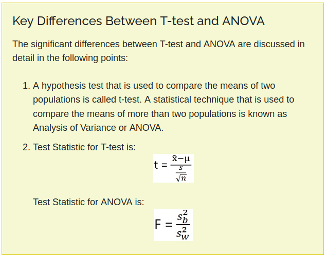
The following diagram summarizes the t-tes and one-way ANOVA.

*In case the above link is broken, click here
Reference:
CHI Square test
The chi-square independence test is a procedure for testing if two categorical variables are related in some population.
There are two types of chi-square tests. Both use the chi-square statistic and distribution for different purposes:
- Goodness of Fit Test: A chi-square goodness of fit test determines if a sample data matches a population.
-
Test for independence: A chi-square test for independence compares two variables in a contingency table to see if they are related. In a more general sense, it tests to see whether distributions of categorical variables differ from each another.
- A very small chi square test statistic means that your observed data fits your expected data extremely well. In other words, there is a relationship, i.e $\chi^2$ is very small.
- A very large chi square test statistic means that the data does not fit very well. In other words, there isn’t a relationship, i.e $\chi^2$ is very large.
- $\chi^2$ = chi squared
- ${O}_i$ = observed value
- $E_{i}$ = expected value
Reference:
Student t-distribution
*In case the above link is broken, click here ![]()
Z-test
population parameters are known
*In case the above link is broken, click here ![]()
More on Z and t statistics
![]() Z test
Z test
population parameters are known
In a z-test, the sample is assumed to be normally distributed.
-
z-test: Here we try to comparesample mean$x$ with population mean $\mu$
A z-score is calculated with population parameters such as population mean and population standard deviation and is used to validate a hypothesis that the sample drawn belongs to the same population.
- Null: Sample mean is same as the population mean
- Alternate: Sample mean is not same as the population mean
The statistics used for this hypothesis testing is called z-statistic, the score for which is calculated as
where
- $x$ = sample mean
- $\mu$ = population mean
- $\frac{\sigma}{\sqrt n}$ = population standard deviation
If the test statistic is lower than the critical value, accept the Alternate Hypothesis or else reject the Alternate hypothesis
![]() t test
t test
-
t-test: Here we try to compare 2sample mean$x_1$ with $x_2$.
A t-test is used to compare the mean of two given samples. Like a z-test, a t-test also assumes a normal distribution of the sample. A t-test is used when the population parameters (mean and standard deviation) are not known.
A t-test is used when the population parameters (mean and standard deviation) are not known.
There are three versions of t-test
-
Independent samples t-test which compares mean for
two groups -
Paired sample t-test which compares means from the same group at
different times -
One sample t-test which tests the mean of a single group against a known mean.
The statistic for this hypothesis testing is called t-statistic, the score for which is calculated as
,where
- $x_1$ = mean of sample 1
- $x_2$ = mean of sample 2
- $n_1$ = size of sample 1
- $n_2$ = size of sample 2
There are multiple variations of t-test which are explained in detail here.
Reference:
Kendall’s Tau (Kendall Rank Correlation Coefficient)
Kendall’s Tau is a non-parametric measure of relationships between columns of ranked data. The Tau correlation coefficient returns a value of 0 to 1, where:
- $0$ is no relationship,
- $1$ is a perfect relationship.
Reference:
How autoML works?
![]() Example: Say if you have a problem of Diabetic Classification and you have different types of data like medical data for Europe, Africa, Asia and you need to build a platform where given any medical history data-set (for any region) it will solve the Diabetic Classification automatically. How to build such platform.
Example: Say if you have a problem of Diabetic Classification and you have different types of data like medical data for Europe, Africa, Asia and you need to build a platform where given any medical history data-set (for any region) it will solve the Diabetic Classification automatically. How to build such platform.
What is AutoML?
Automated Machine Learning provides methods and processes to make Machine Learning available for non-Machine Learning experts, to improve efficiency of Machine Learning and to accelerate research on Machine Learning.
Machine learning (ML) has achieved considerable successes in recent years and an ever-growing number of disciplines rely on it. However, this success crucially relies on human machine learning experts to perform the following tasks:
- Pre-process and clean the data.
- Select and construct appropriate features.
- Select an appropriate model family.
- Optimize model hyperparameters.
- Post-process machine learning models.
- Critically analyze the results obtained.
As the complexity of these tasks is often beyond non-ML-experts, the rapid growth of machine learning applications has created a demand for off-the-shelf machine learning methods that can be used easily and without expert knowledge. We call the resulting research area that targets progressive automation of machine learning AutoML.
![]() Reference:
Reference:
What are the parameters in training a decision tree?
-
max_depth: How deep the tree can be -
min_samples_split: Min number of samples needed to split a node -
min_samples_leaf: Min number of samples needed to be at the leaf node. -
max_features: Max number of features to consider when looking for the best split.
Reference:
What is the philosophy behind Decision Tree?
Tree based methods involve stratifying or segmenting the Predictor space into number of region.
- A decision tree is a tree where each
noderepresents a feature(attribute), eachlink(branch) represents a decision(rule) and eachleafrepresents an outcome(categorical or continues value) - Find the feature that best splits the target class into the
purest possiblechildren nodes (ie: nodes that don’t contain a mix of both classes, rather pure nodes with only one class). -
Entropyon the other hand it is a measure of impurity. It is defined for a classification problem with N classes as: -
Entropy: $-\sum_i c_i * \log(c_i)$, where
i=1,...,N
Say we have a dataset D and we are looking for a potential feature f, on which we will split the dataset w.r.t f into 2 parts Dl and Dr for left and right dataset respectively, such that those two datasets are at their purest form. Finally we use information gain to decide how good that feature is i.e how much pure the split is w.r.t f using Information Gain.
   Df
 /    \
Dl     Dr
-
Information Gain: It is the difference of entropy before the split and after the split.
EntropyBefore_f = Entropy(Df)and entropy after isEntropyAfter_f = Entropy(Dl)+Entropy(Dr)and finalyInformationGain_f = EntropyBefore_f - EntropyAfter_f.
![]() Reference:
Reference:
How to build decision tree?
There are couple of algorithms there to build a decision tree. Some of the important ones are
![]() CART (Classification and Regression Trees) → uses Gini Index(Classification) as metric. Lower the Gini Index, higher the purity of the split.
CART (Classification and Regression Trees) → uses Gini Index(Classification) as metric. Lower the Gini Index, higher the purity of the split.
![]() ID3 (Iterative Dichotomiser 3) → uses Entropy function and Information gain as metrics. Higher the Information Gain, better the split is.
ID3 (Iterative Dichotomiser 3) → uses Entropy function and Information gain as metrics. Higher the Information Gain, better the split is.
What are the criteria for splitting at a node in decision trees ?
Gini Index [link]
- CART uses Gini index as a split metric. For
Nclasses, the Gini Index is defined as: $1-\sum_i p_i^2$, wherei=1,...,Nand $p_i=p(target=i)$ [source]
Information Gain
where,
- $V$ - possible values of categorical feature $A$
- $S$ - set of examples ${X}$
- $S_v$ - subset where $X_A = V$
![]() Cross Entropy
Cross Entropy
-
Cross-entropy loss, or log loss, measures the performance of a classification model whose output is a probability value between $0$ and $1$. - In binary classification, where the number of classes $M=2$, cross-entropy can be calculated as: $-{(y\log(p) + (1 - y)\log(1 - p))}$
- If $M \gt 2$ (i.e. multiclass classification), we calculate a separate loss for each class label per observation and sum the result.
Entropy
![]() CHI Square: It is an algorithm to find out the statistical significance between the differences between sub-nodes and parent node.
CHI Square: It is an algorithm to find out the statistical significance between the differences between sub-nodes and parent node.
Reduction of Variance
:bookmark_Tabs: Reference:
What is the formula of Gini index criteria?
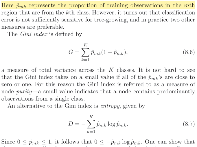
How is it decided that on which features it has to split?
Based on for which feature the information gain is maximum.
![]() Reference:
Reference:
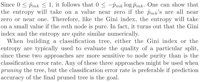
What is the formula for Entropy criteria?
Entropy is the measure of uncertainty; how disordered a system is or in this case, the degree of randomness in a set of data. Higher the entropy, lower the predictability or chances of finding patterns in the data. It can be used to explain the origin of the universe and also where the universe headed towards.
The concept of entropy or the way it is characterised had been implemented in fields remote to thermodynamics.
One such application is determining the limits of carrying out information.
The amount of information that is received as a result of an experiment/activity/event can be considered numerically equivalent to the amount of uncertainty concerning the event.
To characterise entropy and information in a much simpler way, it was initially proposed to consider these quantities as defined on the set of generalised probability distributions.
Entropy is nothing but Expectation with negative sign.
![]() Expectation Formula: $E[g(x)] = \sum p(x)g(x)$
Expectation Formula: $E[g(x)] = \sum p(x)g(x)$
In entropy, $g(x)$ is $\log (p(x))$, and combining with the negative sign (which is apparent as for $0 \leq x \leq 1$ , $\log (x)$ is negative), which makes it positive, the entropy ( or expectation) formula becomes:
![]() NOTE: What entropy doesn’t tell us is the optimal encoding scheme to help us achieve this compression. Optimal encoding of information is a very interesting topic, but not necessary for understanding KL divergence. The key thing with Entropy is that, simply knowing the theoretical lower bound on the number of bits we need, we have a way to quantify exactly how much information is in our data. Now that we can quantify this, we want to quantify how much information is lost when we substitute our observed distribution for a parameterized approximation.
NOTE: What entropy doesn’t tell us is the optimal encoding scheme to help us achieve this compression. Optimal encoding of information is a very interesting topic, but not necessary for understanding KL divergence. The key thing with Entropy is that, simply knowing the theoretical lower bound on the number of bits we need, we have a way to quantify exactly how much information is in our data. Now that we can quantify this, we want to quantify how much information is lost when we substitute our observed distribution for a parameterized approximation.
Reference:
What is KL Divergence?
KL Divergence helps us to measure just how much information we lose when we choose an approximation.
- KL Divergence is the measure of
relative entropy. It is a measure of thedistance between two distributions. - In statistics, it arises as an
expected logarithmof the likelihood ratio.
The relative entropy ${KL}(p\sim||\sim q)$
is a measure of the inefficiency of assuming that the distribution is q, when the true distribution is p.
- Kullback-Leibler Divergence is just a slight modification of our formula for entropy. Rather than just having our probability distribution $p$ we add in our approximating distribution $q$. Then we look at the difference of the log values for each.
- The KL divergence from $p$ to $q$ is simply the difference between cross entropy and entropy:
Where $y_i \sim p$ and $\hat{y}_i \sim q$, i.e. they come from two different probability distribution.
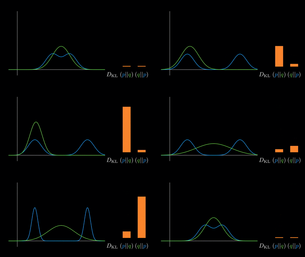
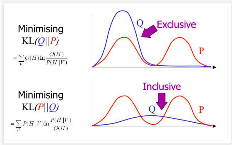
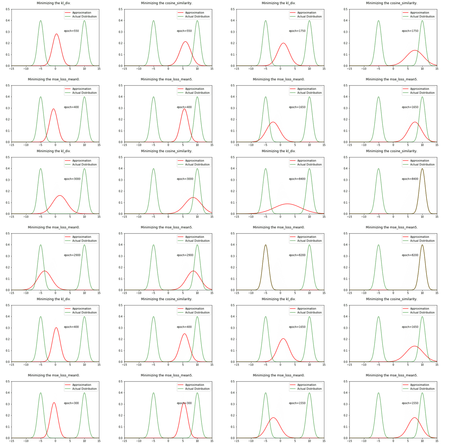
It’s well-known that KL-divergence is not symmetric, but which direction is right for fitting your model?
If we’re fitting $q_{\theta}$ to $p$
- Using $KL(p \vert \vert q_{\theta})$:
Mean-seeking,inclusive(more principled because approximates the full distribution)- Requires normalization wrt p (i.e., often not computationally convenient)
- Using $KL(q_{\theta} \vert \vert p)$:
Mode-seeking,exclusive- No normalization wrt $p$ (i.e., computationally convenient)
Mnemonic: “When the truth comes first, you get the whole truth” Here
whole truthcorresponds to the inclusiveness of $KL(p \vert \vert q)$.
Reference:
-
Kullback-Leibler Divergence Explained

- KL-divergence as an objective function
- Understand KL Divergence
Divergence
In statistics and information geometry,
divergenceor acontrast functionis a function which establishes thedistanceof one probability distribution to the other on a statistical manifold.
The divergence is a weaker notion than that of the distance, in particular the divergence need not be symmetric (that is, in general the divergence from $p$ to $q$ is not equal to the divergence from $q$ to $p$), and need not satisfy the triangle inequality.
The two most important divergences are the
-
Relative entropy(Kullback–Leibler divergence, KL divergence), which is central to information theory and statistics - The
Squared Euclidean distance(SED)
Minimizing these two divergences is the main way that linear inverse problem are solved, via the principle of maximum entropy and least squares, notably in logistic regression and linear regression.
Reference:
Kolmogorov Complexity
Kolmogorov complexity of an object or algorithm is the length of its optimal specification. In some sense, it could be thought of as algorithmic entropy, in the sense that it is the amount of information contained in the object.
Consider the strings
-
11111111111111111111111111111111- it contains 32 1’s - easy to represent -
4c1j5b2p0cv4w1x8rx2y39umgw5q85s7- the best way to describe the other string in haskell is (probably) to just site it
Kolmogorov complexity KKK of a string, relative to a Turing machine fff of a string x,x,x, is
Regerence:
How do you calculate information gain mathematically?
- If
His the entropy of the original data D and it has undergoneNsplits for featuref, then Information Gain:
where i=1,...,N and $S$ is the size of total datasets and $S_i$ is the size of the $i_{th}$ split data.
![]() Reference:
Reference:
Pros and Cons of Decision Trees:
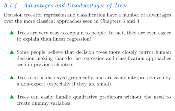
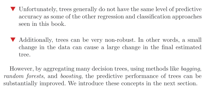
- Decision Tree also suffers from
high variance.
Philosophy behind Bagging?
- Say we have N independent observations $Z_1, \dots Z_N$, each with variance $\sigma^2$. Then the variance of the mean $\bar{Z}$ of the observation is given by $\sigma^2/n$. That is, averaging a set of observations reduce variance.
- Hence a natural way to reduce the variance and hence increase the prediction accuracy of a statistical learning method is to take many training sets from the population, build a separate prediction model using each training set, and average the resulting predictions.
Ensemble methods:

* image source (slide 7)
Reference:
What is the advantage with random forest ?
- Random forest is an ensemble method in which a classifier is constructed by
combining several different Independent base classifiers. - The independence is theoretically enforced by training each base classifier on a training set sampled with replacement from the original training set.
- This technique is known as
bagging, orbootstrap aggregation. - In Random Forest, further randomness is introduced by identifying the best split feature from a random subset of available features.
-
Reduction in overfitting: by averaging several trees, there is a significantly lower risk of overfitting. -
Less variance: By using multiple trees, you reduce the chance of stumbling across a classifier that doesn’t perform well because of the relationship between the train and test data.
Why ensemble is good?
Q: Suppose we have $10$ independent classifiers, each with error rate of $0.3$. What will be the final error rate if we ensemble these $10$ independent classifiers?
$\epsilon=0.3$
In this setting, the error rate of the ensemble can be computed as below:
![]() Assumption: We are taking a majority vote on the predictions.
Assumption: We are taking a majority vote on the predictions.
An ensemble makes a wrong prediction only when more than half of the base classifiers are wrong.
It can be seen that with the theoretical guarantees stated above an ensemble model performs significantly well.
However in practice it is not possible to guarantee such classifier independence as they are trained from the same data, but still introduction of randomness helps achieve independence to a certain degree and it has been empirically observed that ensembles perform significantly well over individual base classifiers.
![]() Reference:
Reference:
Ensemble Learning algorithm
Characteristics of Different Learning Methods
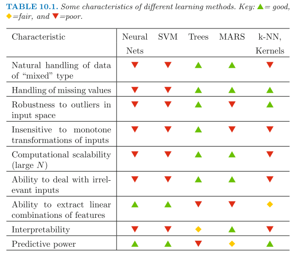
MARS: Multivariate Adaptive Regression Splines
![]() Reference:
Reference:
Boosting algorithms
- For more on boosting algorithm, check here at notion/scribe-ml
The term Boosting refers to a family of algorithms which boosts (i.e converts) weak learner to strong learners.
-
 AdaBoost (Adaptive Boosting)
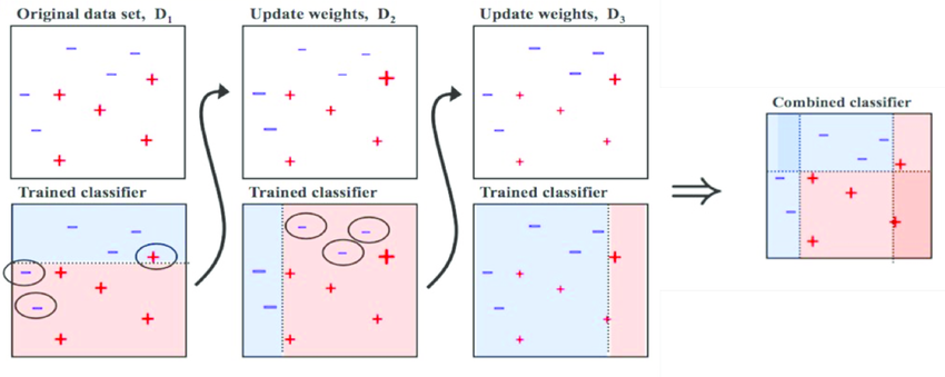
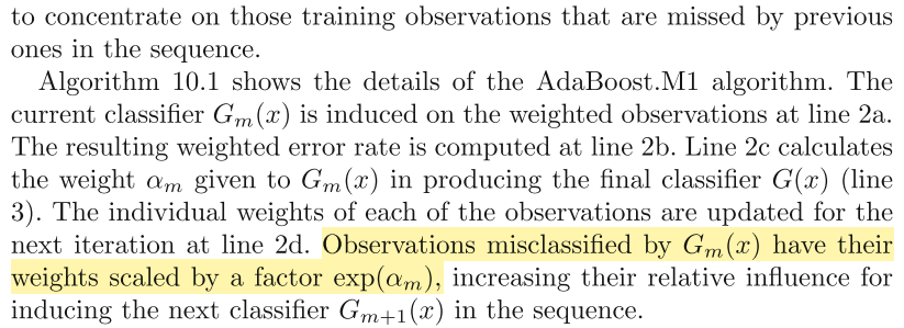
At the end of every model prediction we end up boosting the weights of the misclassified instances so that the next model does a better job on them, and so on.
Adaptive Boosting, or most commonly known AdaBoost, is a Boosting algorithm ![]() . The method this algorithm uses to correct its predecessor is by paying more attention to underfitted training instances by the previous model.
. The method this algorithm uses to correct its predecessor is by paying more attention to underfitted training instances by the previous model.
-
 Gradient Tree Boosting: It works by sequentially adding the previous predictors underfitted predictions to the ensemble, ensuring the erros made previously are corrected.
The difference lies in what it does with the underfitted values of its predecessor.
- AdaBoost: Tweaks the instance weights at every interaction,
- Gradient Boosting: Tries to fit the new predictor to the residual errors made by the previous predictor.
-
 XGBoost: Extreme Gradient Boosting is an advanced implementation of the Gradient Boosting. This algorithm has high predictive power and is ten times faster than any other gradient boosting techniques. Moreover, includes a variety of regularisation which reduces overfitting and improves overall performance.
 -
 Light GB: For datasets which are extremely large Light Gradient Boosting is the best, compared to all of the other, since it takes less time to run.
- The motivation behind the
Boostingalgorithm is, there aren weak classifiers. Combining together gives apowerful committeewho decides the final verdict of the classifier. - A week classifier is one whose error rate is slightly better than
random guessing
![]() Resource:
Resource:
- quick-introduction-boosting-algorithms-machine-learning
- Boosting-with-adaboost-and-gradient-boosting
Do you know about Adaboost algorithm ? How and why does it work ?
![]() AdaBoost:
AdaBoost:
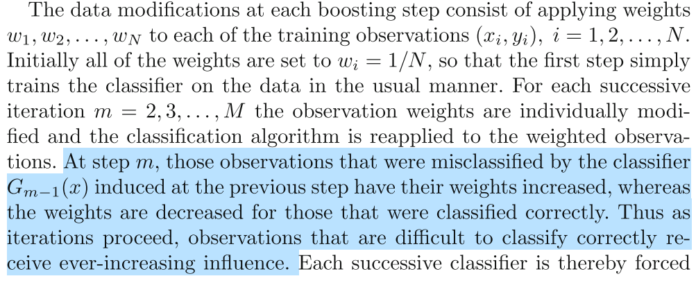
Also called Adaptive Boosting, where boosting is applied in a gradual way in the form of combining new learners on the misclassified data.
- First: A weak learner is applied and all the training examples, which are misclassified, are given higher weight.
- Second: While building the dataset for training the next learner, the previously misclassified training examples will appear in the dataset (as high weight has been given to them). Now on this new dataset another learner is trained. Obviously this learner will correctly classify those previously misclassified examples plus some more misclassification in this step.
- Repeat first and second.
- In AdaBoost you need to define a
base classifier. -
Classification Treeacts as the best off the shelf base classifier for Adaboost.
:bookark_tabs: Resource:
How does gradient boosting works ?
- Bagging and Boosting both are ensemble learning algorithm, where a collection of weak learner builds the strong learner.
- Bagging works on
re-sampling data with replacementand create different dataset and the week learners are learnt on them, and final predictions are taken by averaging or majority voting. E.g. Random Forest.
![]() Bagging: It is a simple ensembling technique in which we build many independent predictors/models/learners on sampled data with replacement from the original data (Bootstrap Aggregation) and combine them using some model averaging techniques. (e.g. weighted average, majority vote or normal average). E.g:
Bagging: It is a simple ensembling technique in which we build many independent predictors/models/learners on sampled data with replacement from the original data (Bootstrap Aggregation) and combine them using some model averaging techniques. (e.g. weighted average, majority vote or normal average). E.g: Random Forest
![]() Boosting: Also an ensemble learning method in which the predictors are not made independently, but sequentially. [link]
Boosting: Also an ensemble learning method in which the predictors are not made independently, but sequentially. [link]
![]() Gradient Boosting:
Gradient Boosting:
- Gradient Boosting is also a boosting algorithm(Duh!), hence it also tries to create a strong learner from an ensemble of weak learners. This is algorithm is similar to Adaptive Boosting (AdaBoost) but differs from it on certain aspects. In this method we try to
visualize the boosting problem as an optimization problem, i.e we take up a loss function and try to optimise it. - We take up a weak learner(in previous case it was decision stump) and at each step, we add another weak learner to increase the performance and build a strong learner. This reduces the loss of the loss function. We iteratively add each model and compute the loss. The loss represents the error residuals(the difference between actual value and predicted value) and using this loss value the predictions are updated to minimise the residuals.
-
 Important: It learns a weak learner $F(x)+\epsilon_1$ ($\epsilon$ is the noise). Then on the noise, i.e. the residual,
it builds another weak learner $H(x)+\epsilon_2$ and so on. Thus it becomes $F(x)+H(x)+G(x)+….+\epsilon$, where $\epsilon = \sum_i \epsilon_i$. Gradient boosting a sequential approach.
![]() Reference:
Reference:
Difference of AdaBoost, Gradient Boost and XGBoost
Both AdaBoost and Gradient Boosting build weak learners in a sequential fashion. Originally, AdaBoost was designed in such a way that at every step the sample distribution was adapted to put more weight on misclassified samples and less weight on correctly classified samples. The final prediction is a weighted average of all the weak learners, where more weight is placed on stronger learners.
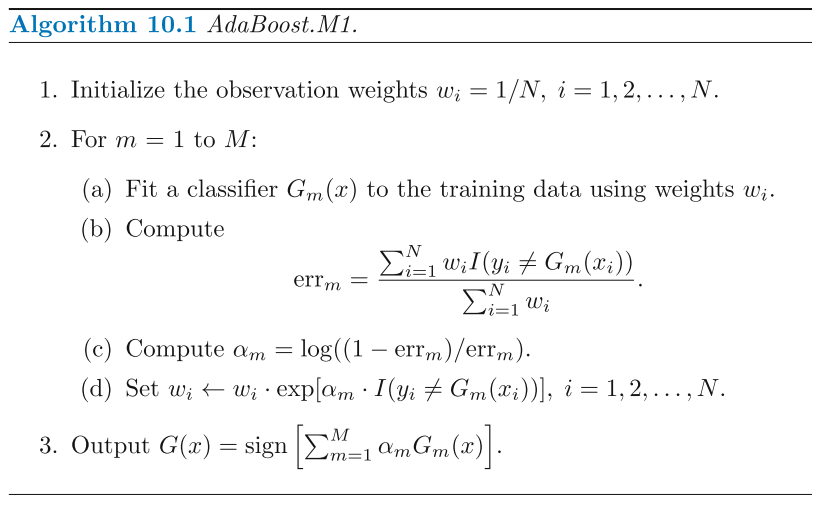
AdaBoost can also be expressed as in terms of the more general framework of additive models with a particular loss function (the exponential loss) [chapter 10 in (Hastie) ESL]. AdaBoost.M1 (Algorithm 10.1, from the book) is equivalent to forward stagewise additive modeling (Algorithm 10.2) using the loss function
In
Gradient Boosting, shortcomings (of existing weak learners) are identified by gradients a.k.a residuals. InAdaboost, ‘shortcomings’ are identified by high-weight data points.
![]() The main differences therefore are that Gradient Boosting is a generic algorithm to find approximate solutions to the additive modeling problem, while AdaBoost can be seen as a special case with a particular loss function. Hence, gradient boosting is much more flexible.
The main differences therefore are that Gradient Boosting is a generic algorithm to find approximate solutions to the additive modeling problem, while AdaBoost can be seen as a special case with a particular loss function. Hence, gradient boosting is much more flexible.
Second, AdaBoost can be interepted from a much more intuitive perspective and can be implemented without the reference to gradients by reweighting the training samples based on classifications from previous learners.
![]() Reference:
Reference:
- Quora: What-is-the-difference-between-gradient-boosting-and-adaboost
- Math Explanation: Imp_link
- Stack Exchange
Bagging boosting difference:
XGBoost: Extreme Gradient Boosting
XGBoost, a scalable machine learning system for tree boosting. The most important factor behind the success of XGBoost is its scalability in all scenarios. The system runs more than ten times faster than existing popular solutions on a single machine and scales to billions of examples in distributed or memory-limited settings.
The scalability of XGBoost is due to several important systems and algorithmic optimizations. These innovations include:
- A novel tree learning algorithm is for handling sparse data
- A theoretically justified weighted quantile sketch procedure enables handling instance weights in approximate tree learning.
- Parallel and distributed computing makes learning faster which enables quicker model exploration.
Objective Function
Read section $2.1$ and $2.2$ of the original XGBoost paper.
![]() Regularized Learning Objective
Regularized Learning Objective
For a given data set with $n$ examples and $m$ features $D = {(x_i, y_i)}$ $( \vert D \vert = n, x_i \in \mathbb{R}^m, y_i \in \mathbb{R})$, a tree ensemble model uses $K$-additive functions to predict the output.
where $f_k \in \mathcal{F}$. Also $\mathcal{F} = {f(\mathbf{x}) = w_{q(\mathbf{x})}}(q : \mathbb{R}^m \rightarrow T, w \in \mathbb{R}^T)$ is the space of regression trees (also known as CART).
- $q$ represents the
structure of each treethat maps an example to the corresponding leaf index. - $T$ is the number of leaves in the tree.
- Each $f_k(.)$ corresponds to an
independent treestructure $q$ and leaf weights $w$. - Unlike decision trees, each regression tree contains a continuous score on each of the leaf, we use $w_i$ to represent score on $i^{th}$ leaf.
For a given example, we will use the decision rules in the trees (given by $q$) to classify it into the leaves and calculate the final prediction by summing up the score in the corresponding leaves (given by $w$). To learn the set of functions used in the model, we minimize the following regularized objective.
where $\Omega(f)= \gamma T + \frac{1}{2} \lambda \vert \vert w \vert \vert^2$, $i$ belongs to all the leaves and $k$ belongs to all the additive functions.
Here $l$ is a differentiable convex loss function that measures the difference between the prediction $\hat{y_i}$ and the target $y_i$. The second term $\Omega$ penalizes the complexity of the model (i.e., the regression tree functions). The additional regularization term helps to smooth the final learnt weights to avoid over-fitting. Intuitively, the regularized objective will tend to select a model employing simple and predictive functions.
![]() NOTE: When the regularization parameter is set to zero, the objective falls back to the traditional gradient tree boosting.
NOTE: When the regularization parameter is set to zero, the objective falls back to the traditional gradient tree boosting.
![]() Gradient Tree Boosting:
Gradient Tree Boosting:
-
Optimization Problem: The tree ensemble model in the above equation includes functions $f_k(.)$ (which is nothing but independent tree structure $q$ with leaf weights $w$) as parameters and cannot be optimized using traditional optimization methods in Euclidean space.
-
Solution: Instead, the model is trained in an additive manner. Formally, let $\hat{y_i}$ be the prediction of the $i^{th}$ instance at the $t^{th}$ iteration, we will need to add $f_t(.)$ to minimize the following objective.
This means we greedily add the $f_t(.)$ that most improves our model according to the above equation. Second-order approximation can be used to quickly optimize the objective in the general setting.
Fore more in-depth math, read the section $2.2$ of the paper.
System design
![]() Column Block for Parallel Learning:
Column Block for Parallel Learning:
The most time consuming part of tree learning is to get
the data into sorted order. In order to reduce the cost of sorting, we propose to store the data in in-memory units, which we called block. Data in each block is stored in the compressed column (CSC) format, with each column sorted by the corresponding feature value. This input data layout only needs to be computed once before training, and can be reused in later iterations.
![]() Cache-aware Access:
Cache-aware Access:
While the proposed block structure helps optimize the computation complexity of split finding, the new algorithm requires indirect fetches of gradient statistics by row index, since these values are accessed in order of feature. This is a non-continuous memory access. A naive implementation of split enumeration introduces immediate read/write de- pendency between the accumulation and the non-continuous memory fetch operation. This slows down split finding when the gradient statistics do not fit into CPU cache and cache miss occur. For the exact greedy algorithm, we can alleviate the problem by a cache-aware prefetching algorithm. Specifically, we allocate an internal buffer in each thread, fetch the gradient statistics into it, and then perform accumulation in a mini-batch manner.
![]() Blocks for Out-of-core Computation:
Blocks for Out-of-core Computation:
One goal of our system is to fully utilize a machine’s re- sources to achieve scalable learning. Besides processors and memory, it is important to utilize disk space to handle data that does not fit into main memory. To enable out-of-core computation, we divide the data into multiple blocks and store each block on disk. During computation, it is important to use an independent thread to pre-fetch the block into a main memory buffer, so computation can happen in concurrence with disk reading.
-
Block Compression: The first technique we use is block compression. The block is compressed by columns, and decompressed on the fly by an independent thread when loading into main memory. This helps to trade some of the computation in decompression with the disk reading cost.
-
Block Sharding: The second technique is to shard the data onto multiple disks in an alternative manner. A pre-fetcher thread is assigned to each disk and fetches the data into an in-memory buffer. The training thread then alternatively reads the data from each buffer. This helps to increase the throughput of disk reading when multiple disks are available.
(SHARD: A database shard is a horizontal partition of data in a database or search engine. Each individual partition is referred to as a shard or database shard. Each shard is held on a separate database server instance, to spread load.)
Reference:
Logistic Regression
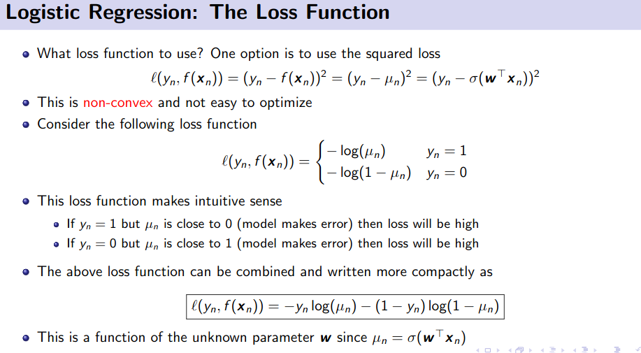
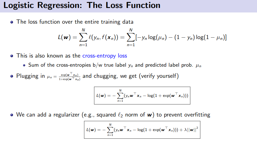
What is the loss function for logistic regression?
This is a very tricky question.
Case 1:
When $y \in ({0,1})$
This is also called cross entropy error function.
Case 2:
When $y \in ({-1,+1})$
Though these 2 equations look different. But if you pay attention for case 1, it’s written in terms of $\hat{y_i}$ but for case 2 there is no such term. Now what is $\hat{y_i}$ ??
So if we substitute this in case 1, then we will find case 2. So they are same.
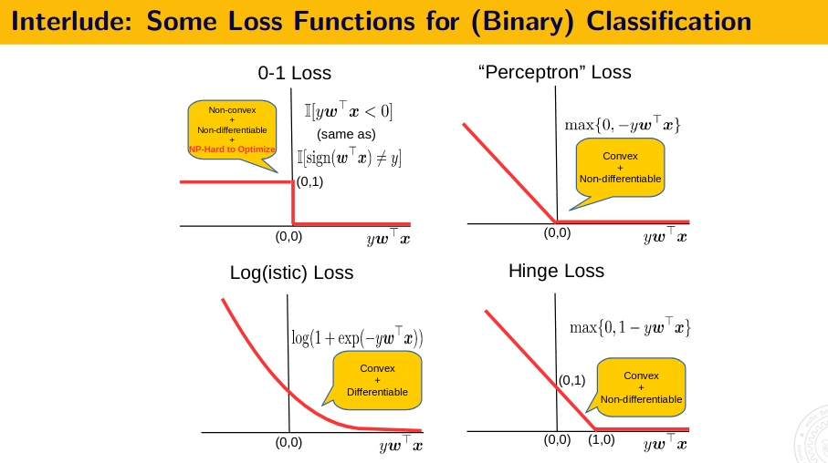
The above image shows, that how we approximate 0-1 loss in SVM and in Logistic regression.
![]() Resource:
Resource:
- Probabilistic Perspective: Murphy - Chapter 8.3.1
- Very IMP, ML Course: Prof. Piyush Rai
- Very IMP, ML Course: Prof. Piyush Rai, slide 13
Comparison of SVM and Logistic Loss?
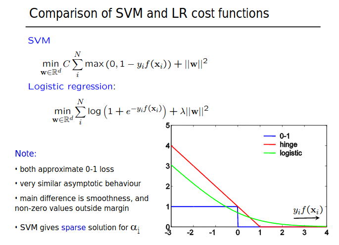
Resource:
Why is logistic regression considered as a linear model?
Q. Is it always necessary the decision boundary is linear / plane always?
The short answer is: Logistic regression is considered a generalized linear model because the outcome always depends on the sum of the inputs and parameters. Or in other words, the output cannot depend on the product (or quotient, etc.) of its parameters! $z = \sum_i w_ix_i$
The key is that our model is additive. Our outcome z depends on the additivity of the weight parameter values, e.g., : $z = w_1x_1 + w_2x_2$
There’s no interaction between the weight parameter values,nothing like $w_1x_1 * w_2x_2$ or so, which would make our model non-linear!
![]() However we can use non-linear feature s.t $z = \sum_i w_if(x_i)$ where $f()$ is a non linear function of $x$. But still $z$ is linear in terms of parameter $w_i$.
However we can use non-linear feature s.t $z = \sum_i w_if(x_i)$ where $f()$ is a non linear function of $x$. But still $z$ is linear in terms of parameter $w_i$.
- In general the decision boundary is linear in
x. To be more specific, the decision boundary in this case is given by $w^Tx=0$ (a hyperplane). But then you go on to saybut we can generate non-linear decision boundaries as well. - Well, of course you can, but then that’ll be called a
non-linear instanceof logistic regression (the exact same way we have linear SVMs and non-linear SVMs). In other words, you can start with your original data x and see/decide that it’s not linearly separable. What you can do next is introduce a feature transformation h(x) and use that in place of x. - For example, if you decide to apply a quadratic feature transformation on say for simplicity, your 2-dimensional data then h(x) in this case is simply given by
$h(x) = [x_1, x_2, x_1^2, x_2^2, x_1x_2]$
and your logistic model is now $y=f(w^Th(x))$ with the decision boundary given by $w^Th(x)=0$ (which is now a
non-linear quadratic curvein the original data space).
![]() Resource
Resource
SVM Summary:
A Support Vector Machine (SVM) performs classification by finding the hyperplane that maximizes the margin between the two classes. The vectors (cases) that define the hyperplane are the support vectors.
Algorithm
- Define an optimal hyperplane: maximize margin
- Extend the above definition for non-linearly separable problems: have a penalty term for misclassifications.
- Map data to high dimensional space where it is easier to classify with linear decision surfaces: reformulate problem so that data is mapped implicitly to this space.
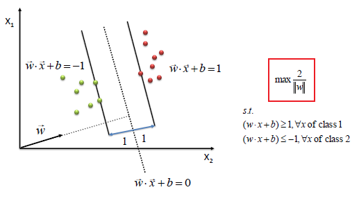
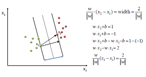
We find w and b by solving the following objective function using Quadratic Programming.
Hard Margin
s.t $y_i(w.x_i+b)\ge 1, \forall x_i$
Soft Margin
The beauty of SVM is that if the data is linearly separable, there is a unique global minimum value. An ideal SVM analysis should produce a hyperplane that completely separates the vectors (cases) into two non-overlapping classes. However, perfect separation may not be possible, or it may result in a model with so many cases that the model does not classify correctly. In this situation SVM finds the hyperplane that maximizes the margin and minimizes the misclassifications.
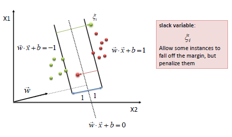
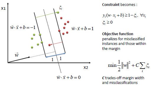
The simplest way to separate two groups of data is with a straight line (1 dimension), flat plane (2 dimensions) or an N-dimensional hyperplane. However, there are situations where a nonlinear region can separate the groups more efficiently. SVM handles this by using a kernel function (nonlinear) to map the data into a different space where a hyperplane (linear) cannot be used to do the separation.
-
It means a non-linear function is learned by a linear learning machine in a high-dimensional feature space while the capacity of the system is controlled by a parameter that does not depend on the dimensionality of the space. This is called kernel trick which means the kernel function transform the data into a higher dimensional feature space to make it possible to perform the linear separation.
Formulate SVM with loss function and solve by gradient decent
![]() Alternative question: How do you adjust the cost parameter for the SVM regularizer?
Alternative question: How do you adjust the cost parameter for the SVM regularizer?
Regularization problems are typically formulated as optimization problems involving the desired objective(classification loss in our case) and a regularization penalty. The regularization penalty is used to help stabilize the minimization of the objective or infuse prior knowledge we might have about desirable solutions. Many machine learning methods can be viewed as regularization methods in this manner. For later utility we will cast SVM optimization problem as a regularization problem.
Re write the soft margin problem using hinge loss $(z)$ defined as the positive part of $1-z$, written as $(1-z)^+$. The relaxed optimization problem (soft margin) can be reformulated as
Here $\frac{1}{2}\vert \vert w \vert \vert^2$, the inverse squared geometric margin is viewed as a regularization penalty that helps stabilizes the objective
What sort of optimization problem would you be solving to train a support vector machine?
-
Maximize Margin(best answer), quadratic program, quadratic with linear constraints, reference to solving the primal or dual form.
What are the kernels used in SVM ?
Kernel $K(X_i, X_j)$ are:
- Linear Kernel: $X_i.X_j$
- Polynomial Kernel: $(\gamma X_i.X_j + C)^d$
- RBF Kernel: $\exp (-\gamma\vert X_i - X_j\vert ^2)$
- Sigmoid Kernel: $\tanh(\gamma X_i.X_j + C)$
where $K(X_i, X_j) = \phi(X_i).\phi(X_j)$
that is, the kernel function, represents a dot product of input data points mapped into the higher dimensional feature space by transformation $\phi(.)$
$\gamma$ is an adjustable parameter of certain kernel functions.
The RBF is by far the most popular choice of kernel types used in Support Vector Machines. This is mainly because of their localized and finite responses across the entire range of the real x-axis.
What is the optimization technique of SVM?
Please download the PDF to view it: Download PDF
Why bring Lagrange Multiplier for solving the SVM problem?
- Constrained Optimization Problem easier to solve with Lagrange Multiplier
- The existing constraints will be replaced by the constraints of the Lagrange Multiplier, which are easier to handle
-
By this
reformulation of the problem, the data will appear only asdot product, which will be very helpful whilegeneralizing the SVM for non linearly separable class. - Youtube:Lagrange Multiplier Intuition
KKT Condition for SVM?
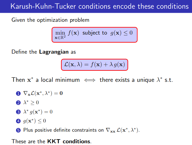
Geometric analysis of Lagrangian, KKT, Dual
How does SVM learns non-linear boundaries ? Explain.
- Using
kernel trick, it maps the examples frominput spacetofeature space. In the higher dimension, they are separated linearly.
SVM: Regularized Loss Function View
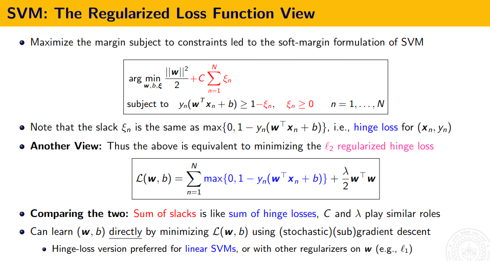
Resource:
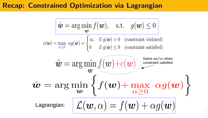
Constrained optimization (Lagrangian)
-
 minimize $f(x)$ such that
 g(x)<=0and $h(x)=0$.- Our target is to bring a new equation where we will combine $f(x), g(x), h(x)$ in a single equation. We will do this by introducing Lagrange Multiplier $\lambda$ and $\mu$. The new equation looks like: $L(x,\lambda,\mu)=f(x)+\lambda g(x)+ \mu h(x)$.
-
 maximize $f(x)$ such that
 g(x)>=0and $h(x)=0$.- Our target is to bring a new equation where we will combine $f(x), g(x), h(x)$ in a single equation. We will do this by introducing Lagrange Multiplier $\lambda$ and $\mu$. The new equation looks like: $L(x,\lambda,\mu)=f(x)+\lambda g(x)+ \mu h(x)$.
NOTE: In the above formulation, pay special attention to the minimize and maximize kewords and the change in inequality constrains. So given any minimization or maximization problem, convert its constraints to $g(x) \leq 0$ or $g(x) \geq 0$ accordingly and then formulate the Lagrangian form. The $h(x)=0$ may or may not be there. Finally apply KKT conditions for finding the solution.
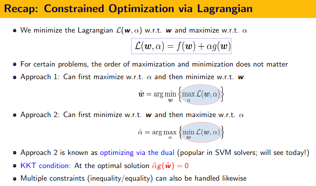
KKT Conditions:
- Stationarity $\nabla_x L(x,\lambda,\mu)=0$
- Primal feasibility, $g(x)<=0$ (for minimization problem)
- Dual feasibility, $\lambda>=0, \mu>=0$
- Complementary slackness, $\lambda g(x) = 0$ and $\mu h(x)=0$
![]() Resource
Resource
Talking about unsupervised learning? What are the algorithms ?
- Clustering
-
K Means
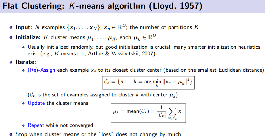
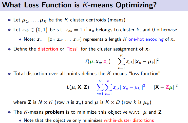
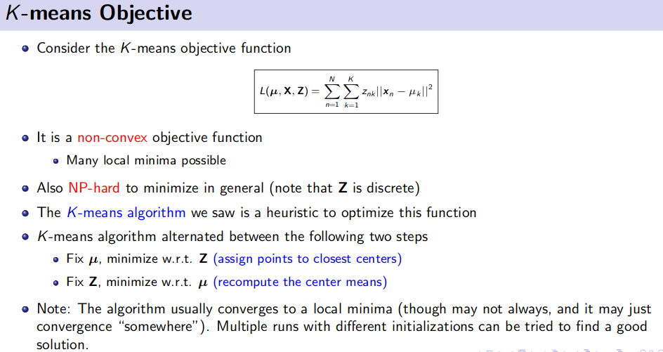
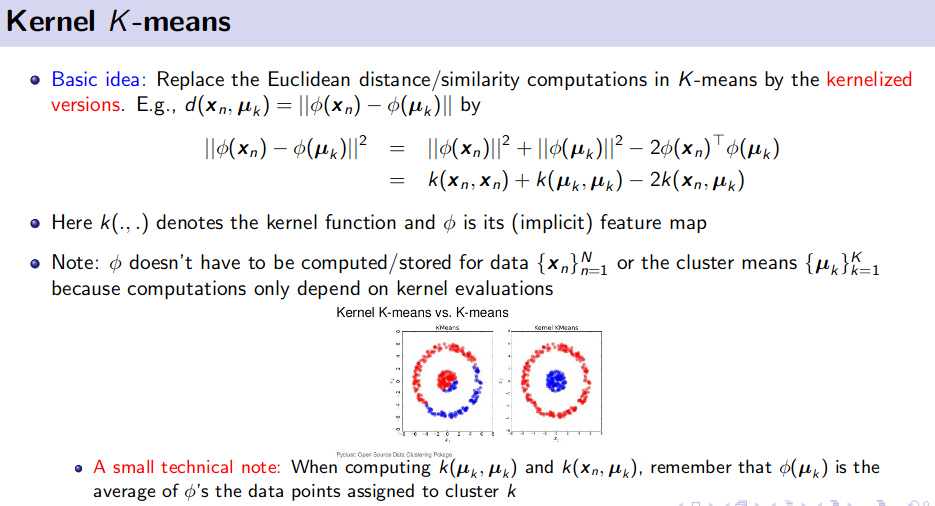
- K-Means clustering intends to partition n objects into k clusters in which each object belongs to the cluster with the nearest mean. This method produces exactly k different clusters of greatest possible distinction. The best number of clusters k leading to the greatest separation (distance) is not known as a priori and must be computed from the data. The objective of K-Means clustering is to minimize total intra-cluster variance, or, the squared error function:
- $J = \Sigma_j \Sigma_i \vert\vert x_i - c_j \vert\vert^2$ where
j=1,...,Kandi=1,...,N.Ntotal number of observations andKtotal number of classes
![]() Resource:
Resource:
![]() Algorithm:
Algorithm:
- Clusters the data into k groups where k is predefined.
- Select k points at random as cluster centers.
- Assign objects to their closest cluster center according to the Euclidean distance function.
- Calculate the centroid or mean of all objects in each cluster.
- Repeat steps b, c and d until the same points are assigned to each cluster in consecutive rounds.
-
Seed K-Means: For seeding, i.e, to decide the insitial set of
Kcentroids, use K-Means++ algorithm. - K Medoids
- Agglomerative Clustering
- Hierarchichal Clustering
- Dimensionality Reduction
- PCA
- ICA
How do you decide K in K-Means clustering algorithm ?Tell me at least
3 ways of deciding K in clustering ?
- Elbow Method
- Average Silhouette Method
- Gap Statistics
![]() Reference:
Reference:
How do you seed k-means algorithm,i.e. how to decide the first k clusters?
-
k-means++is an algorithm for choosing the initial values (or “seeds”) for the k-means clustering algorithm. It was proposed in 2007 by David Arthur and Sergei Vassilvitskii, as an approximation algorithm for theNP-hard k-meansproblem - a way of avoiding the sometimes poor clustering found by the standard k-means algorithm. - The intuition behind this approach is that spreading out the k initial cluster centers is a good thing: the first cluster center is chosen uniformly at random from the data points that are being clustered, after which each subsequent cluster center is chosen from the remaining data points with probability proportional to its squared distance from the point’s closest existing cluster center.
- The exact algorithm is as follows:
Algorithm
- Choose one center uniformly at random from among the data points.
- For each data point x, compute D(x), the distance between x and the nearest center that has already been chosen.
- Choose one new data point at random as a new center, using a weighted probability distribution where a point x is chosen with probability proportional to D(x)^2.
- Repeat Steps 2 and 3 until k centers have been chosen.
- Now that the initial centers have been chosen, proceed using standard k-means clustering.
![]() Reference:
Reference:
When K-means will fail?
- When data is non linearly separable. It works best when data clusters are discrete and spherically distributed.
What other clustering algorithms do you know?
- link
- Unsupervised linear clustering algorithm
- k-means clustering algorithm link
- Fuzzy c-means clustering algorithm
- Hierarchical clustering algorithm
- Hierarchical Agglomerative Clustering (bottom up)
- Hierarchical DIvisive Clustering (top down)
- Gaussian(EM) clustering algorithm
- Quality threshold clustering algorithm
- Unsupervised non-linear clustering algorithm
-
MST based clustering algorithm
- Basic Idea: Apply MST on the data points. Use the Euclidean distance as the weight between two data points. After building the MST removes the longest edge, then the 2nd longest and so on. And thus clusters will be formed. source
- kernel k-means clustering algorithm
- Density based clustering algorithm
- DBSCAN
- code
What is DB-SCAN algorithm ?
- It is a density-based clustering algorithm: given a set of points in some space, it groups together points that are closely packed together (points with many nearby neighbors), marking as outliers points that lie alone in low-density regions
- A point p is a core point if at least
minPtspoints are within distanceε(εis the maximum radius of the neighborhood from p) of it (including p). Those points are said to be directly reachable from p. - A point q is
directly reachablefrom p if point q is within distanceεfrom point p and p must be a core point. - A point q is
reachablefrom p if there is a pathp1, ..., pnwithp1 = pandpn = q, where eachpi+1is directly reachable frompi(all the points on the path must be core points, with the possible exception of q). - All points not reachable from any other point are outliers.
How does HAC (Hierarchical Agglomerative clustering) work ?
The Inductive Biases of Various Machine Learning Algorithms
That is, there is some fundamental assumption or set of assumptions that the learner makes about the target function that enables it to generalize beyond the training data
Linear Regression
- The relationship between the attributes x and the output y is linear. The goal is to minimize the sum of squared errors.
Decision Trees
- Shorter trees are preferred over longer trees. Trees that place high information gain attributes close to the root are preferred over those that do not.
Single-Unit Perceptron:
- Each input votes independently toward the final classification (interactions between inputs are not possible).
Neural Networks with Backpropagation:
- Smooth interpolation between data points.
K-Nearest Neighbors:
- The classification of an instance x will be most similar to the classification of other instances that are nearby in Euclidean distance.
Support Vector Machines:
- Distinct classes tend to be separated by wide margins.
Naive Bayes:
- Each input depends only on the output class or label; the inputs are independent from each other.
Reference:
How do you deploy Machine Learning models ?
- Microservice
- Docker
- Kubernetes
Lot of times, we may have to write ML models from scratch in C++ ? Will you be able to do that?
How the model varies in KNN for $K=1$ and $K=N$?
- When K equals 1 or other small number the model is prone to
overfitting (high variance), while when K equals number of data points or other large number the model is prone tounderfitting (high bias).
Generative model vs Discriminative model.
-
Discriminative algorithms model
P(y|x; w), that is, given the dataset and learned parameter, what is the probability of y belonging to a specific class. A discriminative algorithm doesn’t care about how the data was generated, it simply categorizes a given example. -
Generative algorithms try to model
P(x|y), that is, the distribution of features given that it belongs to a certain class. A generative algorithm models how the data was generated. source
Scenario based Question
Let’s say, you are given a scenario where you have terabytes of data files consisting of pdfs, text files, images, scanned pdfs etc. What approach will you take in understanding or classifying them ?
Q. How will you read the content of scanned pdfs or written documents in image formats?
Why is naive bayes called “naive”? Tell me about naive bayes classifier?
- Because it’s assumed that all the features are independent of each other. This is a very naive assumption.
Logistic Regression loss function?
What do you mean by mutable and immutable objects in python ?
Since everything in Python is an Object, every variable holds an object instance. When an object is initiated, it is assigned a unique object id. Its type is defined at runtime and once set can never change, however its state can be changed if it is mutable. Simple put, a mutable object can be changed after it is created, and an immutable object can’t.
- Objects of built-in types like (
int, float, complex, bool, str, tuple, unicode, frozen set) are immutable. Objects of built-in types like (list, set, dict,byte array) are mutable. Custom classes are generally mutable.
What are the data structures you have used in python ?
Difference between Multi-Class and Multi-Label classification
Multi-Class Classification
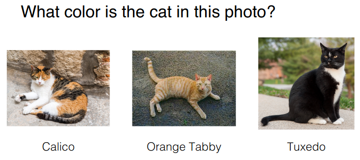
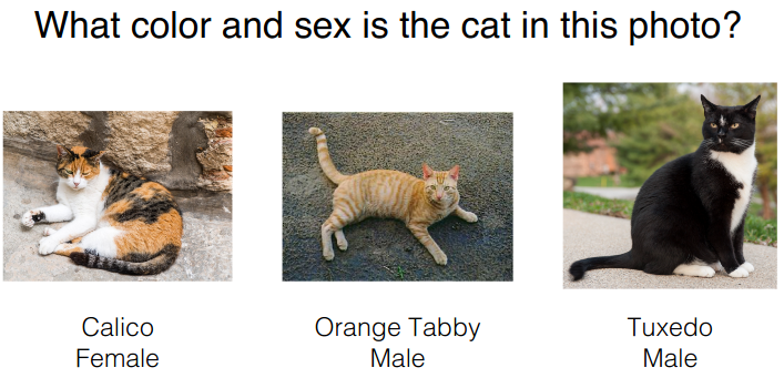
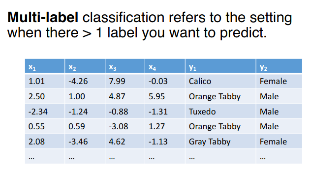
Multi-Label Classification
Method:
- Not so good idea: Two independent classifiers might output combinations of labels that don’t make sense.
Limitations:
- Calico cats are almost always female
- If your classifiers predict male and calico, this is probably wrong
- There might be correlations between the classes that you could help classification if you had a way to combine the two classifiers
- Good idea: train one classifier first, use its output as a feature in the other.
Limitations:
- If the first classifier is wrong, you’ll have an incorrect feature value.
- This is a
pipelineapproach where one classifier informs the other, rather than both informing each other simultaneously.
- Better Idea: treat combinations of classes as their own “classes”, then do single-label classification. combine Class $y_1$ and $y_2$ and create single class and use multi-class classification.
Limitations:
- All classes are learned independently:the classifier has no idea that
Tuxedo+MaleandTuxedo+Femaleare both the same color and therefore probably have similar feature weights.
![]() Reference:
Reference:
How do you handle multi-class classification with unbalanced dataset ?
- link1
- handling imbalanced data by resampling original data to provide balanced classes.
- Random under sampling
- Random over sampling
- Cluster based over sampling
- Informed Over Sampling: Synthetic Minority Over-sampling Technique (SMOTE)
- Modifying existing classification algorithms to make them appropriate for imbalanced data sets.
- Bagging based
- Boosting based: AdaBoost, Gradient Boost, XGBoost
- imp source
How do you select between 2 models (Model Selection techniques)?
To choose between 2 model generally AIC or BIC are used.
Generally, the most commonly used metrics, for measuring regression model quality and for comparing models, are: Adjusted R2, AIC, BIC and Cp.
-
AIC stands for (Akaike’s Information Criteria), a metric developped by the Japanese Statistician, Hirotugu Akaike, 1970. The basic idea of AIC is to
penalize the inclusion of additional variablesto a model. It adds a penalty that increases the error when including additional terms.The lower the AIC, the better the model.AICcis a version of AIC corrected for small sample sizes. - BIC (or Bayesian information criteria) is a variant of AIC with a stronger penalty for including additional variables to the model.
-
 Mallows Cp: A variant of AIC developed by Colin Mallows
 - $R^2$ not a good criterion.Always increase with model size –>
optimumis to take the biggest model. -
Adjusted$R^2$: better. Itpenalizedbigger models.
![]() Reference:
Reference:
How does it work mathematically? Explain the intuition behind BIC or AIC ?
In general, it might be best to use AIC and BIC together in model selection.
-
For example, in selecting the number of latent classes in a model, if BIC points to a three-class model and AIC points to a five-class model, it makes sense to select from models with 3, 4 and 5 latent classes.
-
AIC is better in situations when a false negative finding would be considered more misleading than a false positive, -
BIC is better in situations where a false positive is as misleading as, or more misleading than, a false negative.
where,
- $\theta$= the set (vector) of model parameters
- $L(\theta)$ = the likelihood of the candidate model given the data when evaluated at the maximum likelihood estimate of $\theta$
- $k$ = the number of estimated parameters in the candidate model
The first compo-nent, $−2\log L(\hat \theta)$, is the value of the likelihood function, $\log L(\theta)$, which is the probability of obtaining the data given the candidate model. The more parameters, the greater the amount added to the first component, increasing the value for the AIC and penalizing the model.
BIC is another model selection criterion based on infor-mation theory but set within a Bayesian context. The difference between the BIC and the AIC is the greater penalty imposed for the number of param-eters by the BIC than the AIC.
Reference:
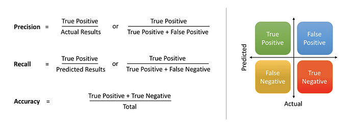
What is precision and recall? Which one of this do you think is important in medical diagnosis?
Type I and Type II Errors
One fine morning, Jack got a phone call. It was a stranger on the line. Jack, still sipping his freshly brewed morning coffee, was barely in a position to understand what was coming for him. The stranger said, “Congratulations Jack! You have won a lottery of $10$ Million USD! I just need you to provide me your bank account details, and the money will be deposited in your bank account right way…”
What are the odds of that happening? What should Jack do? What would you have done?

- Type I: False Positive
- Type II: False Negative
ROC Curve Analysis
ROC curve
An ROC curve (receiver operating characteristic curve) is a graph showing the performance of a classification model at all classification thresholds. This curve plots two parameters:
- True Positive Rate:
- True Positive Rate (TPR) is a synonym for recall and is therefore defined as follows:
- False Positive Rate
To compute the points in an ROC curve, we could evaluate a logistic regression model many times with different classification thresholds, but this would be inefficient. Fortunately, there’s an efficient, sorting-based algorithm that can provide this information for us, called AUC.
AUC: Area Under the ROC Curve
AUC stands for “Area under the ROC Curve.” That is, AUC measures the entire two-dimensional area underneath the entire ROC curve (think integral calculus) from (0,0) to (1,1).
AUC provides an aggregate measure of performance across all possible classification thresholds. One way of interpreting AUC is as the probability that the model ranks a random positive example more highly than a random negative example. (source)
What does AUC-ROC curve signify ?
AUC - ROC curve is a performance measurement for classification problem at various thresholds settings. ROC is a probability curve and AUC represents degree or measure of separability. It tells how much model is capable of distinguishing between classes. Higher the AUC, better the model is at predicting 0s as 0s and 1s as 1s. By analogy, Higher the AUC, better the model is at distinguishing between patients with disease and no disease.
How do you draw AUC-ROC curve ?
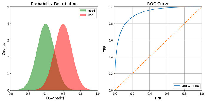
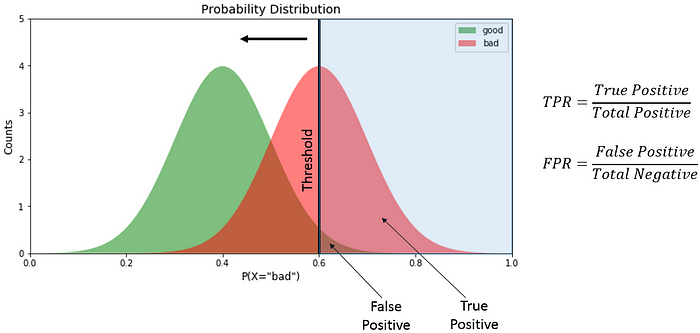
-
True positiveis the area designated as “bad” on the right side of the threshold (mild sky blue region).False positivedenotes the area designated as “good” on the right of the threshold. -
Total positiveis the total area under the “bad” curve while total negative is the total area under the “good” curve. - We divide the value as shown in the diagram to derive TPR and FPR.
- We derive the TPR and FPR at different threshold values (by sliding the black vertical bar in the above image) to get the ROC curve. Using this knowledge, we create the ROC plot function.
Bonus Question: Write pseudo-code to generate the data for such a curve. [Check the below blog]
The ROC curve is plotted with TPR against the FPR where TPR is on y-axis and FPR is on the x-axis.

TPR == RECALL
- Specificity:
FPR == 1-Specificity
How will you draw ROC for multi class classification problem
In multi-class model, we can plot N number of AUC ROC Curves for N number classes using One vs ALL methodology. So for Example, If you have three classes named X, Y and Z, you will have one ROC for X classified against Y and Z, another ROC for Y classified against X and Z, and a third one of Z classified against Y and X.
Reference
What is random about Random Forest?
- For different
tree, a different datasets (build from original using random resampling with replacement) are given as input.
Metric to measure multi-class classification result?
We can generalize all the binary performance metrics such as precision, recall, and F1-score etc. to multi-class settings. In the binary case, we have:
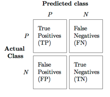
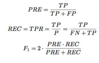

And to generalize this to multi-class, assuming we have a One-vs-All (OvA) classifier, we can either go with the micro average or the macro average.
-
Micro averaging: we’d calculate the performance, e.g., precision, from theindividual(assuming One-vs-All) true positives, true negatives, false positives, and false negatives of the the k-class model:

Macro-averaging: We average the performances of each individual class.

Reference:
How is using a logistic regression different from using a random forest ?
- If your data is linearly separable, go with logistic regression. However, in real world, data is rarely linearly separable. Most of the time data would be a jumbled mess. In such scenarios, Decision trees would be a better fit as DT essentially is a non-linear classifier. As DT is prone to over fitting, Random Forests are used in practice to better generalize the fitment. RF provide a good balance between precision and overfitting.
- If your problem/data is linearly separable, then first try logistic regression. If you don’t know, then still start with logistic regression because that will be your baseline, followed by non-linear classifier such as random forest. Do not forget to tune the parameters of logistic regression / random forest for maximizing their performance on your data.
- If your data is categorical, then random forest should be your first choice; however, logistic regression can be dealt with categorical data.
- If you want to understand results easily, logistic regression is a better choice because it leads to simple interpretation of the explanatory variables.
- If
speedis your criteria, thenlogistic regressionshould be your choice. - If your
dataisunbalanced, thenrandom forestmay be a better choice. - If number of data objects are less than the number of features, logistic regression should not be used.
- Lastly, as noted in this paper, either of the random forest or logistic regression “models appear to perform similarly across the datasets with performance more influenced by choice of dataset rather than model selection”
![]() Reference:
Reference:
Which model would you use in case of unbalanced dataset: Random Forest or Boosting ? Why ?
- Gradient boosting is also a good choice here. You can use the gradient boosting classifier in sci-kit learn for example. Gradient boosting is a principled method of dealing with class imbalance by constructing successive training sets based on incorrectly classified examples.
- link1
- An alternative could be a cost-sensitive algorithm like C5.0 that doesn’t need balanced data. You could also think about applying Markov chains to your problem.
How to prepare for ML Interview?
In general, for an interview that you think will be machine learning focused, I would make sure you knew the following techniques, and an approach you would use for each, and how they are different from each other:
- Regression
- Classification
- Ranking
- Recommendation
- Clustering
- Unsupervised Learning
Question source:
Exercise
- What is sensitivity and specificity ?
- Name the package of scikit-learn that implements logistic regression ?
- What is mean and variance of standard normal distribution ?
- What is central limit theoram?
- Law of Large Number?
-
What are the data structures you have used in python ?
- What is naive bayes classifier ?
- What is the probability of heads coming 4 times when a coin is tossed 10 number of times ?
- How do you get an index of an element of a list in python ?
- How do you merge two data-set with pandas?
frames = [df1, df2, df3]
result = pd.concat(frames)
- From user behavior, you need to model fraudulent activity. How are you going to solve this ? May be anomaly detection problem or a classification problem !!
-
What will you prefer a decision tree or a random forest ?
- Will you use decision tree or random forest for a classification problem ? What is advantage of using random forest ?
-
- What are the boosting techniques you know ?
- Which model would you like to choose if you have many classes in a supervised learning problem ? Say 40-50 classes !!
- How do you perform ensemble technique?
- How does SVM work ?
- What is Kernel ? Explain a few.
- How do you perform non-linear regression?
- What are Lasso and Ridge regression ?
- What is Gaussian Mixture model ? How does it perform clustering ?
- How is Expectation Maximization performed ? Explain both the steps ?
- How is likelihood calculated in GMM ?