Practical Deep Learning (CV)

Content

Content
How to fine-tune pre-trained model in Computer Vision?
1. Image Data Augmentation
2. How should my classifier look like?

How to fine-tune pre-trained model in Computer Vision?

For full details reading this blog is a must.

However I am sharing some basic techniques from the blog rest you can follow the original blog.

Image Data Augmentation

This is one of those parts where you really have to test and visualize how the image looks. It’s obviously a tricky task to get it right so let’s think about how we could go about it. Points to consider:

Are we doing enough data augmentation?
Are we doing too much?

One of the easiest ways to go about it is to work with the simple transforms from PyTorch such as RandomRotation or ColorJitter.

data_transform = transforms.Compose([
    	transforms.RandomRotation(25),
    	transforms.RandomResizedCrop(224),
    	transforms.ToTensor(),
    	transforms.Normalize([0.485, 0.456, 0.406],
                         	[0.229, 0.224, 0.225])])

Content

How should my classifier look like?

This section is very important

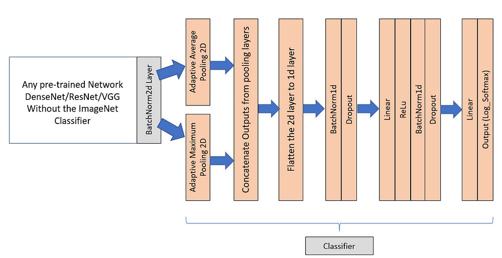
Generally in the transfer learning tasks the Fully Connected (FC) classifier layers are ripped off and new FC layers are added to train on the new data and perform the new task. But many students would generally stick with the conventional Linear and Dropout layers in the FC layers. Could we add some different layers? Yes we could, consider the following example where we added AdaptivePooling Layers in the new classifier:

class Flatten(nn.Module):
    def forward(self, input):
        return input.view(input.size(0), -1)
      
class ClassifierNew(nn.Module):
    def __init__(self, inp = 2208, h1=1024, out = 102, d=0.35):
        super().__init__()
        self.ap = nn.AdaptiveAvgPool2d((1,1))
        self.mp = nn.AdaptiveMaxPool2d((1,1))
        self.fla = Flatten()
        self.bn0 = nn.BatchNorm1d(inp*2,eps=1e-05, momentum=0.1, affine=True)
        self.dropout0 = nn.Dropout(d)
        self.fc1 = nn.Linear(inp*2, h1)
        self.bn1 = nn.BatchNorm1d(h1,eps=1e-05, momentum=0.1, affine=True)
        self.dropout1 = nn.Dropout(d)
        self.fc2 = nn.Linear(h1, out)
        
    def forward(self, x):
        ap = self.ap(x)
        mp = self.mp(x)
        x = torch.cat((ap,mp),dim=1)
        x = self.fla(x)
        x = self.bn0(x)
        x = self.dropout0(x)
        x = F.relu(self.fc1(x))
        x = self.bn1(x)
        x = self.dropout1(x)         
        x = self.fc2(x)
        
        return x

This is how the architecture will look like

For more architecture tuning follow this kaggle notes

In the above example we have added AdaptiveMaxPool2d and AdaptiveAveragePool2d and flattened them out and concatenated them to form a linear layer of size -1 x 2* size(Last BatchNorm2d Layer).

For example in DenseNet161:

The last BacthNorm2d layer has an output dimension of -1x2208x7x7
After passing the mini-batch through the 2 Adaptive Pooling layers we obtain 2 output tensors of shape -1x2208x1x1
Concatenation of the above 2 tensors would result in a tensor of shape -1x4416x1x1
Finally flattening the tensor of shape -1x4416x1x1 would result a Liner Layer of -1x4416 i.e (-1x2*(2208))
This layer is then connected to the Fully Connected part
Note: -1 in the above tensor shapes should be replaced with the mini-batch size

Reason: Why we did this? It could be attributed to the pooling layers because they capture richer features from the convolutional layers and we need to provide them as best as possible to the Classifier so they could classify easily and this would also effectively reduce the number of linear layers we need. This implementation is outlined is fast.ai library (A higher level API for PyTorch), we just re-implemented it here.

Also use other improvements like

Learning Rate Annealing / Scheduling
Improved Optimizer
Unfreezing layers selectively
Weight Decay [interesting idea]

Reference:

Content

Published on August 3, 2019