Reinforcement Learning
Content
- Content
- Beginner’s Guide:
- Multi Arm bandit
- How can we design a systematic strategy that adapts to these stochastic rewards?
- Bandit Problem
- Application of Bandit Algorithm
- Online Learning
- Counterfactual Regret Minimization
- Reinforcement Learning
- CTR
- Exercise:
Beginner’s Guide:
- Blog: A Beginner’s Guide to Deep Reinforcement Learning
- Blog:An introduction to Q-Learning: Reinforcement Learning
- Blog: Introduction to Reinforcement Learning
- AV: A Hands-On Introduction to Deep Q-Learning using OpenAI Gym in Python
Multi Arm bandit
The multi-armed bandit problem is a classic problem that well demonstrates the exploration vs exploitation dilemma. Imagine you are in a casino facing multiple slot machines and each is configured with an unknown probability of how likely you can get a reward at one play. The question is: What is the best strategy to achieve highest long-term rewards?
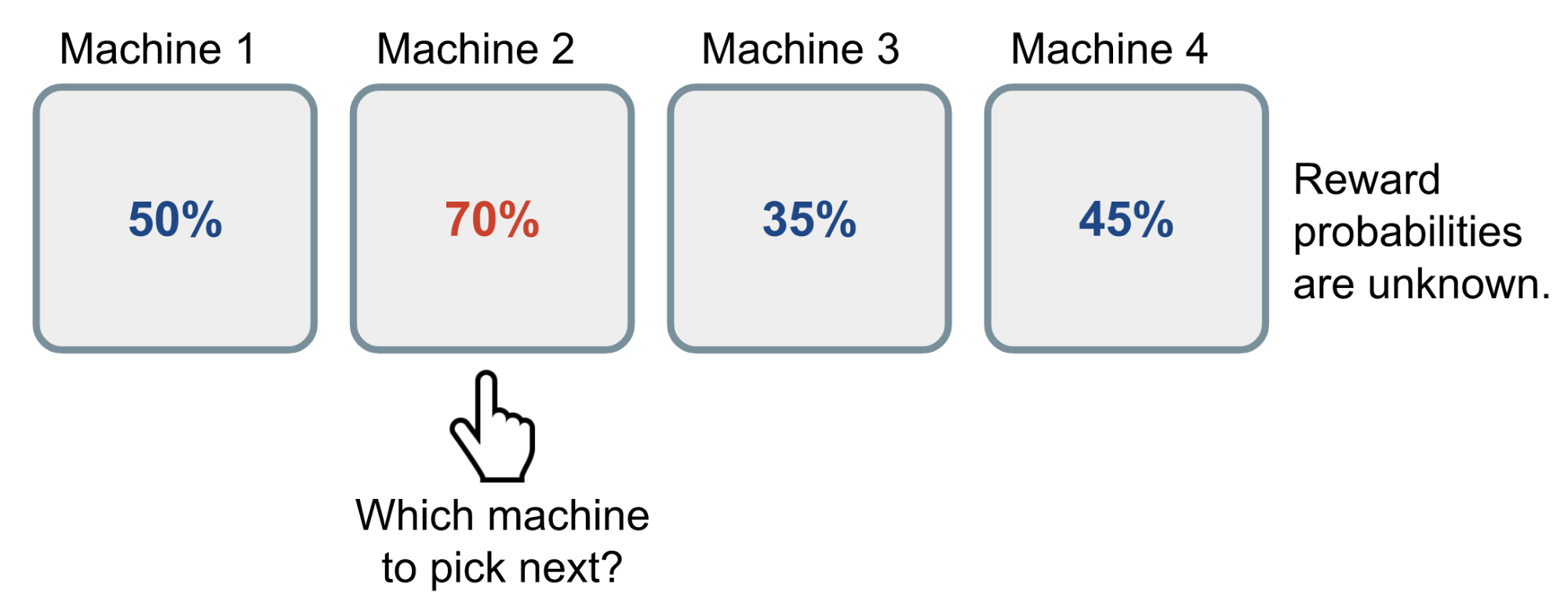
A naive approach can be that you continue to playing with one machine for many many rounds so as to eventually estimate the “true” reward probability according to the law of large numbers. However, this is quite wasteful and surely does not guarantee the best long-term reward.
Reference:
- Book
- Youtube: Exploitation vs Exploration
- Important Blog
- Regret Analysis of Stochastic and Non-stochastic Multi-armedBandit Problems
- Blog
- IITM: CS6046: Multi-armed bandits
- AV: Reinforcement Learning Guide: Solving the Multi-Armed Bandit Problem from Scratch in Python
- The Multi-Armed Bandit Problem and Its Solutions
How can we design a systematic strategy that adapts to these stochastic rewards?
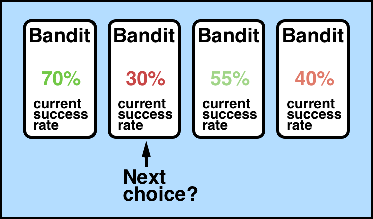
This is our goal for the multi-armed bandit problem, and having such a strategy would prove very useful in many real-world situations where one would like to select the “best” bandit out of a group of bandits i.e. A/B testing, line-up optimization, evaluating social media influence.
we approach the multi-armed bandit problem with a classical reinforcement learning technique of an epsilon-greedy agent with a learning framework of reward-average sampling to compute the action-value $Q(a)$ to help the agent improve its future action decisions for long-term reward maximization.
Reference:
Bandit Problem
This tutorial intends to be an introduction to stochastic and adversarial multi-armed bandit algorithms and to survey some of the recent advances. In the multi-armed bandit problem, at each stage, an agent (or decision maker) chooses one action (or arm), and receives a reward from it. The agent aims at maximizing his rewards. Since he does not know the process generating the rewards, he needs to explore (try) the different actions and yet, exploit (concentrate its draws on) the seemingly most rewarding arms.
Let’s say the Bandit had $K$ arms and $N$ rounds.
- if $K \lt N$: Small set of actions
- if $K \gt N$: Large set of actions
Reference:
Application of Bandit Algorithm
- Clinical trials/dose discovery
- Recommendation systems (movies/news/etc)
- Advert placement
- A/B testing
- Network routing
- Dynamic pricing (eg., for Amazon products)
- Waiting problems (when to auto-logout your computer)
- Ranking (eg., for search)
- A component of game-playing algorithms (MCTS)
- Resource allocation
- A way of isolating one interesting part of reinforcement learning
Reference:
Online Learning
An important area with a rich literature and multiple connections with game theory and optimization that is increasingly influencing the theoretical and algorithmic advances in machine learning.
- The online scenario involves multiple rounds where training and testing phases are intermixed.
- At each round, the learner receives an unlabeled training point, makes a prediction, receives the true label, and incurs a loss.
- The objective in the on-line setting is to minimize the cumulative loss over all rounds or to minimize the regret, that is the difference of the cumulative loss incurred and that of the best expert in hindsight (i.e with experience).
- Unlike the traditional ML settings, no distributional assumption is made in on-line learning. In fact, instances and their labels may be chosen adversarially within this scenario.
- These algorithms process one sample at a time with an update per iteration that is often computationally cheap and easy to implement.
# No distributional assumption.
# Worst-case analysis (adversarial).
# Mixed training and test.
# Performance measure: mistake model, regret.
Similar Problems
- Route selection (internet, traffic).
- Games (chess, backgammon).
- Stock value prediction.
- Decision making
How Online learning is different from traditional machine learning?
Traditional machine learning (PAC learning) follows the key assumption that the distribution over data points is fixed over time, both for training and test points, and that points are sampled in an i.i.d. fashion. Under this assumption, the natural goal is to learn a hypothesis with a small expected loss or generalization error.
In contrast, with on-line learning, no distributional assumption is made, and thus there is no notion of generalization. Instead, the performance of on-line learning algorithms is measured using a mistake model and the notion of regret.
What is Regret?
Definition: The regret at time $T$ is the difference between the loss incurred up to $T$ by the algorithm and that of the best expert in hindsight:
for best regret minimization algorithms: $R_T \leq O(\sqrt{T \log N})$
*expert in hindsight: means the expert learns with more experiment
Prediction with expert advice
In this setting, at the $t$ th round, in addition to receiving $x_t \in X,$ the algorithm also receives advice $y_{t,i} \in Y, i \in [N],$ from $N$ experts. Following the general framework of on-line algorithms, it then makes a prediction, receives the true label and incurs a loss. After $T$ rounds, the algorithm has incurred a cumulative loss. The objective in this setting is to minimize the regret $R_T$, also called external regret, which compares the cumulative loss of the algorithm to that of the best expert in hindsight after $T$ rounds:
Conclusion
On-line learning, regret minimization:
- rich branch of machine learning.
- connections with game theory.
- simple and minimal assumptions.
- algorithms easy to implement.
- scale to very large data sets.
Reference:
- Using Online Learning Algorithms for Computational Advertising
- Book: Foundation of Machine Learning by Mehryar Mohri
Counterfactual Regret Minimization
Reference:
Reinforcement Learning
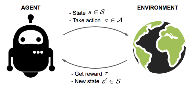
- The training and testing phases are also intermixed in reinforcement learning.
- To collect information, the learner actively interacts with the environment and in some cases affects the environment, and receives an immediate reward for each action.
- The object of the learner is to maximize his reward over a course of actions and iterations with the environment.
- However, no long-term reward feedback is provided by the environment, and the learner is faced with the exploration versus exploitation dilemma, since he must choose between exploring unknown actions to gain more information versus exploiting the information already collected.
Reference:
- My Journey to Reinforcement Learning — Part 2: Multi-Armed Bandit Problem
- Book: Foundation of Machine Learning by Mehryar Mohri
CTR
What is Click Through Rate?
It can be thought of as the number of times the link is clicked by the user divided by the total number of times it’s viewed by the user.
Reference:
- Paper: Beyond the Click-Through Rate: Web Link Selection with Multi-level Feedback
- optimise-ad-ctr-with-reinforcement-learning
CTR Prediction
Motivation: The key task for a search engine advertising system is to
- Determine what advertisements should be displayed from a pool of advertisement
- In what order
for each query that the search engine receives.
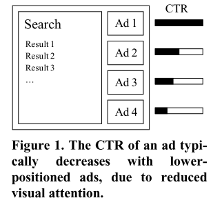
Typically, advertisers have already specified the circumstances under which their ads may be shown (e.g., only for certain queries, or when certain words appear in a query), so the search engine only needs to rank the reduced set of ads that are matches [1].
As with search results, the probability that a user clicks on an advertisement declines rapidly, as much as $90\%$, with display position.
The number of eligible advertisements matching a given query usually far exceeds the number of valuable slots.
As per [13],
- The core of CTR prediction problem is a simple regression. We have a feature vector, usually sparse, that we use to predict the outcome of an interaction, in this case the probability of a click.
- An ad’s CTR is basically the average probability of a click of each impression of the ad. Having a binary click/no-click classification is not enough as the real-world system we have the problem we are solving is selecting an ad from a set of candidate ads, and the reasonable way to make that selection is to predict how likely each one of them is to yield a click and pick the one with the highest probability.
- An easy model will be logistic regression which will give a probability between 0 and 1. Though in the year 2007, people used this kind of model but not now.
- Currently more meaningful model will be anything related to
online learningorreinforcement learning.
Data pattern
- Historical bidding and Engagement Data
- Semantic analysis of the campaign materials
- Campaign id
- Ad’s past performance
- Ad id
- Semantic profile of the ad campaign material
- Timestamp
- Ad placement id
- Site domain
- Media name / ID
- Page URL
- Bid amount
- User context data
- Country where the request originated from
- City where the request originated from
- The type of device used
Highly imbalanced data:
- 1 click data against 2000 non-clicked data
Useful definition:
- Buyer: Someone who has ads to show and money to pay for it. [Example: Nike, Addidas]
-
Clear Price: The final price for the impression (i.e. for displaying the ad.).
-
First price auction: This is the price the winner of the auction bid -
Second price auction:it is the second place bid plus one cent.
-
- Impression: The displaying of the ad in the user’s browser.
- Click Through Rate: The rate at which users click an ad. Nowadays it is usually around 0.06% or so.
- Cost-Per-Acquisition (CPA): The price the advertiser pays for each customer acquired.
-
Cost-Per-Impression (CPI): The most common basic pricing method of online advertising. The advertiser pays for each impression their ad is shown to a user. The price is usually given as thousand impressions,
cost per milleor CPM. - Cost-Per-Click (CPC): The price the advertiser pays for every user clicking on their ad. $CPC=(CPM*CTR)/1000$
- Pay-Per-Click (PPC): A billing method where the advertiser pays for each time a user clicks the ad. In the pay-per-click (PPC) model, the click price is predetermined and is indicated as CPC (Cost Per Click).
- Placement: The actual ad frame or similar. Also known as the tag. This is usually a piece of JavaScript code that adds an iframe element to the page in question. The iframe contents are the actual ad that are loaded from the ad exchange.
- Exchange: An ad server that can do an auction between different buyers/DSPs (demand side platform) and select the ad to send to seller. Some notable exchanges are AppNexus and Google DoubleClick.
-
Real Time Bidding (RTB): A digital ad delivery system where the ad impression on a webpage is sold in an auction just as it is being displayed (the “Real Time” in RTB), and the buyers in the auction decide the price they will bid as it happens based on any information they have about the user and
placementof the particular impressions.
The RTB process in brief:
- A user browses a page with ads
- Ad placement code loads and requests an ad from an exchange
- Exchange requests bids from DSPs (demand side platform, i.e. from different buyers)
- Each buyer decides what they want to bid for the impression based on different kinds of criteria including, but not limited, to user profile, ad profile, placement profile etc
- Exchange picks the highest bid(s) that meet some internal criteria (such as image size, text length, text content etc.) and sends it forward to the placement
- Ad is shown in the placement and a beacon pixel is fired to notify the buyer, usually with the final impression price.
Modelling
In order to maximize ad quality (as measured by user clicks) and total revenue, most search engines today order their ads primarily based on expected revenue:
Thus, to ideally order a set of ads, it is important to be able to accurately estimate the $p(click)*(CTR)$ for a given ad. For ads that have been shown to users many times (ads that have many impressions), this estimate is simply the binomial MLE (maximum likelihood estimation), $n_{clicks} / n_{impressions}$.
Whenever an ad is displayed on the search results page, it has some chance of being seen by the user. The farther down the page an ad is displayed, the less likely it is to be viewed. As a simplification, we consider the probability that an ad is clicked on to be dependent on two factors:
- The probability that it is viewed
- The probability that it is clicked on, given that it is viewed:
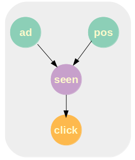
Goal: To create a model which can predict this $p(click \vert ad, pos)$ for new ads.
Simple Model
According to [1], we can model them with simple logistic regression as follows:
where $Z= \Sigma_i w_i f_i(ad)$, where $f_i(ad)$ is the value of the $i^{th}$ feature for the ad, and $w_i$ is the learned weight for that feature. Features may be anything, such as the number of words in the title, the existence of a word, etc.
The logistic regression was trained using the limited-memory Broyden-Fletcher-Goldfarb-Shanno (L-BFGS) method. Use a cross-entropy loss function, with zero-mean Gaussian weight priors with a standard-deviation of $\sigma$. For more details read the paper [1].
![]() Reference:
Reference:
- [1] ** Base Paper 2007: Predicting Clicks: Estimating the Click-Through Rate for New Ads
- [2] An Effective Budget Management Framework for Real-time Bidding in Online Advertising
- [3] A CTR prediction model based on user interest via attention mechanism
- [4] A Context-Aware Click Model for Web Search
- [5] WSDM 2020: Interpretable Click-Through Rate Prediction through Hierarchical Attention
- [6] Learning Compositional, Visual and Relational Representations for CTR Prediction in Sponsored Search
- [7] TOIS 2019: Constructing Click Model for Mobile Search with Viewport Time
- [8] Improving Ad Click Prediction by Considering Non-displayed Events
- [9] KDD 2019: Generating Better Search Engine Text Advertisements with Deep Reinforcement Learning
- [10] **Selecting multiple web adverts: A contextual multiarmed bandit with state uncertainty
- [11] KDD 2013: Ad Click Prediction: a View from the Trenches - from **Google
- [12] ADKDD 2014: Practical Lessons from Predicting Clicks on Ads at Facebook
- [13] Thesis 2019: Click-Through Rate Prediction in Practice by Kurt-Eerik Ståhlberg4
- [14] **JMLR 2013: Counterfactual Reasoning and Learning Systems: The Example of Computational Advertising
** must read papers
Exercise:
- What is PAC learning? [Foundations of Machine Learning by Mehryar Mohri]
- What is Counterfactual Regret Minimization (Source)
- How online learning algorithms are connected to game theory
- What is game theory and min-max algorithm