Content

1. Content
2. Introduction
3. What is Permutation Importance
   1. Code Example
4. Partial Dependence Plots
   1. How it Works
5. How does LIME work?
6. How does SHapley Additive exPlanations (SHAP) work?
   1. Additive Feature Attribution Methods
   2. Classic Shapley Value Estimation
   3. Simple Properties Uniquely Determine Additive Feature Attributions

Introduction

Understanding why a model makes a certain prediction can be as crucial as the prediction’s accuracy in many applications. However, the highest accuracy for large modern datasets is often achieved by complex models that even experts struggle to interpret, such as ensemble or deep learning models, creating a tension between accuracy and interpretability.

There are different kinds of model explainability

• Global Feature Explainability
  • Feature Selection while model building
  • Permutation Importance
  • Partial Dependency
• Local Feature Explainability
  • LIME
  • SHAP

This kaggle blog has nice and easy examples for clear understanding.

What is Permutation Importance

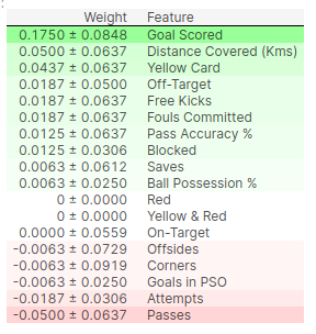
Permutation importance is calculated after a model has been fitted. So we won’t change the model or change what predictions we’d get for a given value of height, sock-count, etc.

Instead we will ask the following question: If I randomly shuffle a single column of the validation data, leaving the target and all other columns in place, how would that affect the accuracy of predictions in that now-shuffled data?

Code Example

import eli5
from eli5.sklearn import PermutationImportance

perm = PermutationImportance(my_model, random_state=1).fit(val_X, val_y)
eli5.show_weights(perm, feature_names = val_X.columns.tolist())

Content

Partial Dependence Plots

While feature importance shows what variables most affect predictions, partial dependence plots show how a feature affects predictions.

This is useful to answer questions like:

• Controlling for all other house features, what impact do longitude and latitude have on home prices? To restate this, how would similarly sized houses be priced in different areas?
• Are predicted health differences between two groups due to differences in their diets, or due to some other factor?

If you are familiar with linear or logistic regression models, partial dependence plots can be interpreted similarly to the coefficients in those models. Though, partial dependence plots on sophisticated models can capture more complex patterns than coefficients from simple models. If you aren’t familiar with linear or logistic regressions, don’t worry about this comparison.

How it Works

Like permutation importance, partial dependence plots are calculated after a model has been fit. The model is fit on real data that has not been artificially manipulated in any way.

Here is the code to create the Partial Dependence Plot using the PDPBox library.

from matplotlib import pyplot as plt
from pdpbox import pdp, get_dataset, info_plots

# Create the data that we will plot
pdp_goals = pdp.pdp_isolate(model=sklearn_tree_model, dataset=val_X, model_features=feature_names, feature='Goal Scored')

# plot it
pdp.pdp_plot(pdp_goals, 'Goal Scored')
plt.show()

Explanation: A few items are worth pointing out as you interpret this plot

1. The y axis is interpreted as change in the prediction from what it would be predicted at the baseline or leftmost value.
2. A blue shaded area indicates level of confidence

From this particular graph, we see that scoring a goal substantially increases your chances of winning “Man of The Match.” But extra goals beyond that appear to have little impact on predictions.

Content

How does LIME work?

The LIME method interprets individual model predictions based on locally approximating the model around a given prediction.

The local linear explanation model that LIME uses adheres to the below equation and is thus an additive feature attribution method.

LIME refers to simplified inputs $x’$ as interpretable inputs, and the mapping $x = h_x(x’)$ converts a binary vector of interpretable inputs into the original input space.

Different types of $h_x$ mappings are used for different input spaces.

• For bag of words text features, $h_x()$ converts a vector of $1$’s or $0$’s (present or not) into the original word count if the simplified input is one, or zero if the simplified input is zero.
• For images, $h_x()$ treats the image as a set of super pixels; it then maps $1$ to leaving the super pixel as its original value and $0$ to replacing the super pixel with an average of neighboring pixels (this is meant to represent being missing).

To find $\phi$, LIME minimizes the following objective function:

Faithfulness of the explanation model $g(z’)$ to the original model $f(hx(z’))$ is enforced through the loss $L$ over a set of samples in the simplified input space weighted by the local kernel $\pi_x$. $\Omega$ penalizes the complexity of $g$. Since in LIME $g$ follows Equation $1$ and $L$ is a squared loss, Equation $2$ can be solved using penalized linear regression.

Content

How does SHapley Additive exPlanations (SHAP) work?

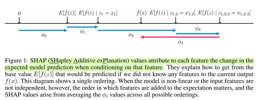
SHAP presents a unified framework for interpreting predictions. SHAP assigns each feature an importance value for a particular prediction. Its novel components include: (1) the identification of a new class of additive feature importance measures, and (2) theoretical results showing there is a unique solution in this class with a set of desirable properties. The

Additive Feature Attribution Methods

The best explanation of a simple model is the model itself; it perfectly represents itself and is easy to understand. For complex models, such as ensemble methods or deep networks, we cannot use the original model as its own best explanation because it is not easy to understand. Instead, we must use a simpler explanation model, which we define as any interpretable approximation of the original model.

Let f be the original prediction model to be explained and $g$ the explanation model. Here, we focus on local methods designed to explain a prediction f(x) based on a single input $x$, as proposed in LIME.

Definition 1 Additive feature attribution methods have an explanation model that is a linear function ofbinary variables:

</center>

$ g(z) = \phi_0 + \sum\limits_{i=1}^{M}\phi_i z_{i}’ $

</center>

where $z’ \in {0, 1}^M$, $M$ is the number of simplified input features, and $\phi_i ∈ \mathbb{R}$.

Methods with explanation models matching Definition 1 attributes an effect $\phi_i$ to each feature, and summing the effects of all feature attributions approximates the output $f(x)$ of the original model. Many current methods match Definition 1.

Classic Shapley Value Estimation

Shapley regression values are feature importance for linear models in the presence of multi-collinearity. This method requires retraining the model on all feature subsets $S \subseteq F$, where $F$ is the set of all features.

It assigns an importance value to each feature that represents the effect on the model prediction of including that feature. To compute this effect, a model $f_{S \cup {i}}(.)$ is trained with that feature present, and another model $f_S(.)$ is trained with the feature withheld.

Then, predictions from the two models are compared on the current input $f_{S \cup {i}}(x_{S∪{i}}) − f_S(x_S)$, where $x_S$ represents the values of the input features in the set $S$.

Since the effect of withholding a feature depends on other features in the model, the preceding differences are computed for all possible subsets $S \subseteq F /\ {i}$. The Shapley values are then computed and used as feature attributions. They are a weighted average of all possible differences:

Simple Properties Uniquely Determine Additive Feature Attributions

A surprising attribute of the class of additive feature attribution methods is the presence of a single unique solution in this class with three desirable properties (described below). While these properties are familiar to the classical Shapley value estimation methods, they were previously unknown for other additive feature attribution methods.

Property 1 (Local accuracy)

The explanation model $g(x’)$ matches the original model $f(x)$ when $x = h_x(x’)$, where $\phi_0 = f(h_x(\mathbf{0}))$ represents the model output with all simplified inputs toggled off(i.e. missing).

Property 2 (Missingness)

Missingness constrains features where $x’_i = 0$ to have no attributed impact.

Property 3 (Consistency)

Let $f_x(z’) = f(h_x(z’))$ and $z’ \backslash i$ denote setting $z’_i = 0$. For any two models $f$ and $f’$, if

for all inputs $z’ \in {0, 1}^M$, then $\phi_i(f’, x) \geq \phi_i(f, x)$.

Note: LIME uses only property 1, where as SHAP combines 1-3 all, more powerful, robust and generic.

Theorem 1 Only one possible explanation model $g$ follows Definition 1 and satisfies Properties 1, 2, and 3:

where $\vert z’ \vert$ is the number of non-zero entries in $z’$, and $z’ \subseteq x’$ represents all $z’$ vectors where the non-zero entries are a subset of the non-zero entries in $x’$.

Theorem 1 follows from combined cooperative game theory results, where the values $\phi_i$ are known as Shapley values.

Note: LIME perturbs the input data to create neighbour input space for getting a local explanation. But SHAP uses the idea of additive feature, whether to include a feature or not. Not including a feature is missing feature here.

Now whether to set missing feature with zero or with other values,it needs some background information. So in the SHAP API, to create the explainer you need to provide some background data, not necessarily the training data.

Reference:

• Paper SHAP: A Unified Approach to Interpreting Model Predictions, NIPS 2017
• Paper LIME: “Why Should I Trust You?”Explaining the Predictions of Any Classifier, KDD2016

Back to Top