DISCLAIMER: I am not the original author of these contents. I compile from various sources to understand a concept and for future reference as I believe in DRY (Don’t Repeat Yourself !!). This blog is nothing but a SCRIBE for me. Solely for education purposes. I try my best to put all the due credits in the reference. If you find any content is incorrect or credit is missing, please contact me. I will be happy to add/edit them.

---

Content

1. Content
2. Introduction
3. Attention High Level
   1. How to Compute Attention Score?
4. Transformer - Visual Understanding
   1. Why Transformer is more suitable than RNN based model?
   2. Self-Attention: the “Look at Each Other” Part
   3. Self-Attention in Detail
   4. Query, Key, and Value in Self-Attention
   5. Matrix Calculation of Self-Attention
   6. Masked Self-Attention: “Don’t Look Ahead” for the Decoder
   7. But how can the decoder look ahead?
   8. Multi Headed Attention: Independently Focus on Different Things
   9. Positional Encoding
   10. The Residuals
   11. The Decoder Side
5. Transformer - Deeper Understanding
   1. Comapre Transformer with Seq2Seq model
   2. Multi-Head Attention
   3. Multi-Head Self-Attention: What are these heads doing?
   4. The Most Important Heads are Interpretable
   5. Position-wise Feed-Forward Networks
   6. Add and Norm
   7. Positional Encoding
   8. What is position wise FFN?
   9. Encoder
   10. Decoder
6. Subword Segmentation: Byte Pair Encoding
   1. Dealing with rare words
   2. The Origins of Byte Pair Encoding
   3. Repurposing BPE for Subword Tokenization
   4. Training: learn BPE rules
   5. Inference: segment a text
   6. What makes BPE the secret sauce?
7. How does Attention Work ?
   1. Attention
   2. Encoder-Decoder with Attention
   3. More on Attention
   4. What is Transformer and it’s pros and cons?
8. Attention is All You Need
   1. Positional Encoding
   2. Transformer Machine Translation
   3. Transformer Language Pre-training
   4. Multi-head attention
9. Machine Translation, seq2seq model
   1. Encoder-Decoder Model
   2. Neural Machine Translation (NMT)

---

Introduction

… in classic seq2seq model, encoder RNN passes the last hidden state as context_vector to the decoder. But in Attention model, the encoder RNN passes all the hidden states to the decoder and takes linear combination of all the encoder hidden states…

From the blog of Jay Alammar

Sequence-to-sequence models are deep learning models that have achieved a lot of success in tasks like machine translation, text summarization, and image captioning. Google Translate started using such a model in production in late 2016. These models are explained in the two pioneering papers (Sutskever et al. 2014, Cho et al., 2014).

In neural machine translation, a sequence is a series of words, processed one after another. The output is, likewise, a series of words:

Under the hood, the model is composed of an encoder and a decoder.

The encoder processes each item in the input sequence, it compiles the information it captures into a vector (called the context). After processing the entire input sequence, the encoder sends the context over to the decoder, which begins producing the output sequence item by item.

The context is nothing but a vector of floats. It is basically the number of hidden units in the encoder RNN.

The context vector turned out to be a bottleneck for these types of models. It made it challenging for the models to deal with long sentences. A solution was proposed in Bahdanau et al., 2014 and Luong et al., 2015. These papers introduced and refined a technique called Attention, which highly improved the quality of machine translation systems. Attention allows the model to focus on the relevant parts of the input sequence as needed.

An attention model differs from a classic sequence-to-sequence model in two main ways:

First, the encoder passes a lot more data to the decoder. Instead of passing the last hidden state of the encoding stage, the encoder passes all the hidden states to the decoder:

Attention mechanism takes a linear combination of all the encoder hidden states

Second, an attention decoder does an extra step before producing its output. In order to focus on the parts of the input that are relevant to this decoding time step, the decoder does the following:

• Look at the set of encoder hidden states it received – each encoder hidden states is most associated with a certain word in the input sentence
• Give each hidden states a score (let’s ignore how the scoring is done for now)
• Multiply each hidden states by its softmaxed score, thus amplifying hidden states with high scores, and drowning out hidden states with low scores

The attention-mechanism looks at an input sequence and decides at each step which other parts of the sequence are important.

Neural networks, in particular recurrent neural networks (RNNs), are now at the core of the leading approaches to language understanding tasks such as language modeling, machine translation and question answering.

In Attention Is All You Need, the authors introduce the Transformer, a novel neural network architecture based on a self-attention mechanism that we believe to be particularly well suited for language understanding.

In the paper, the author shows that the Transformer outperforms both recurrent and convolutional models on academic English to German and English to French translation benchmarks. On top of higher translation quality, the Transformer requires less computation to train and is a much better fit for modern machine learning hardware, speeding up training by up to an order of magnitude.

The sequence-to-sequence neural network models are widely used for NLP. A popular type of these models is an encoder-decoder. There, one part of the network — encoder — encodes the input sequence into a fixed-length context vector. This vector is an internal representation of the text. This context vector is then decoded into the output sequence by the decoder. See an example:

However, there is a catch with the common encoder-decoder approach: a neural network compresses all the information of an input source sentence into a fixed-length vector. It has been shown that this leads to a decline in performance when dealing with long sentences. The attention mechanism was introduced by Bahdanau in “Neural Machine Translation by Jointly Learning to Align and Translate” to alleviate this problem.

Reference:

• Attention Explained by Jay Alammar MUST read

---

Attention High Level

An attention mechanism is a part of a neural network. At each decoder step, it decides which source parts are more important. In this setting, the encoder does not have to compress the whole source into a single vector - it gives representations for all source tokens (for example, all RNN states instead of the last one).

*image source

*image source

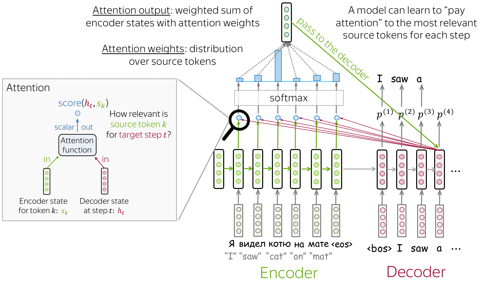
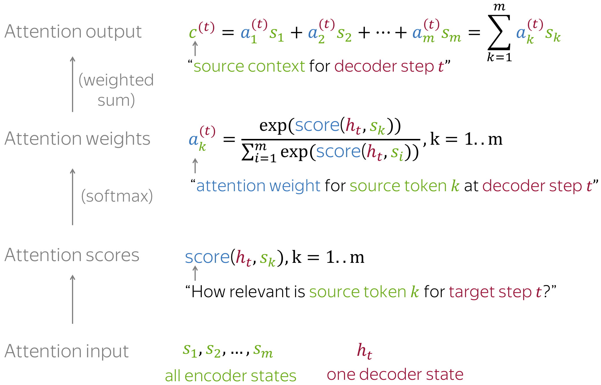
Everything is differentiable - learned end-to-end! The main idea that a network can learn which input parts are more important at each step. Since everything here is differentiable (attention function, softmax, and all the rest), a model with attention can be trained end-to-end. You don’t need to specifically teach the model to pick the words you want - the model itself will learn to pick important information.

How to Compute Attention Score?

In the general pipeline above, we haven’t specified how exactly we compute attention scores. You can apply any function you want - even a very complicated one. However, usually you don’t need to - there are several popular and simple variants which work quite well.

Most popular is Bahdanau Model

• encoder: bidirectional
• To better encoder each source word, the encoder has two RNNs, forward and backward, which read input in the opposite directions. For each token, states of the two RNNs are concatenated.
• attention score: multi-layer perceptron
• To get an attention score, apply a multi-layer perceptron (MLP) to an encoder state and a decoder state. attention applied: between decoder steps
• Attention is used between decoder steps: state $h_{t-1}$ is used to compute attention and its output $c^{(t)}$ , and both $h_{t-1}$ and $c^{(t)}$ are passed to the decoder at step $t$ .

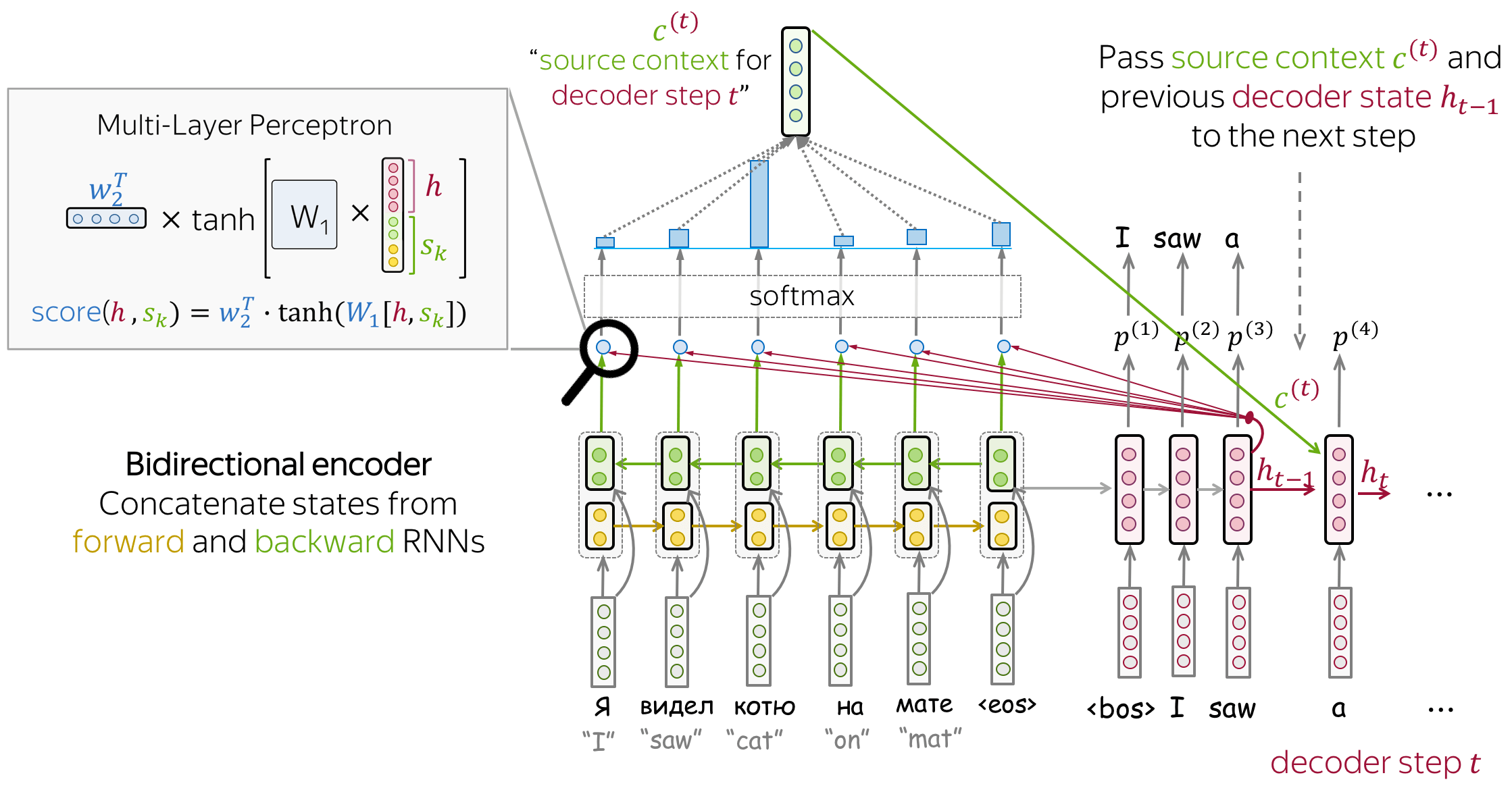
observe the color coding for different vectors

Reference:

• Attention: A High-Level View - Lena Voita

---

Transformer - Visual Understanding

The transformer has no recurrent or convolutional structure, even with the positional encoding added to the embedding vector, the sequential order is only weakly incorporated. For problems sensitive to the positional dependency like reinforcement learning, this can be a big problem.

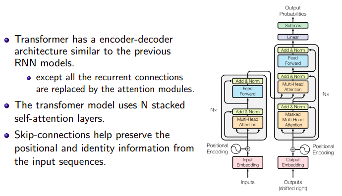
It presented a lot of improvements to the soft attention and make it possible to do seq2seq modeling without recurrent network units. The proposed transformer model is entirely built on the self-attention mechanisms (scaled dot product attention) without using sequence-aligned recurrent architecture.

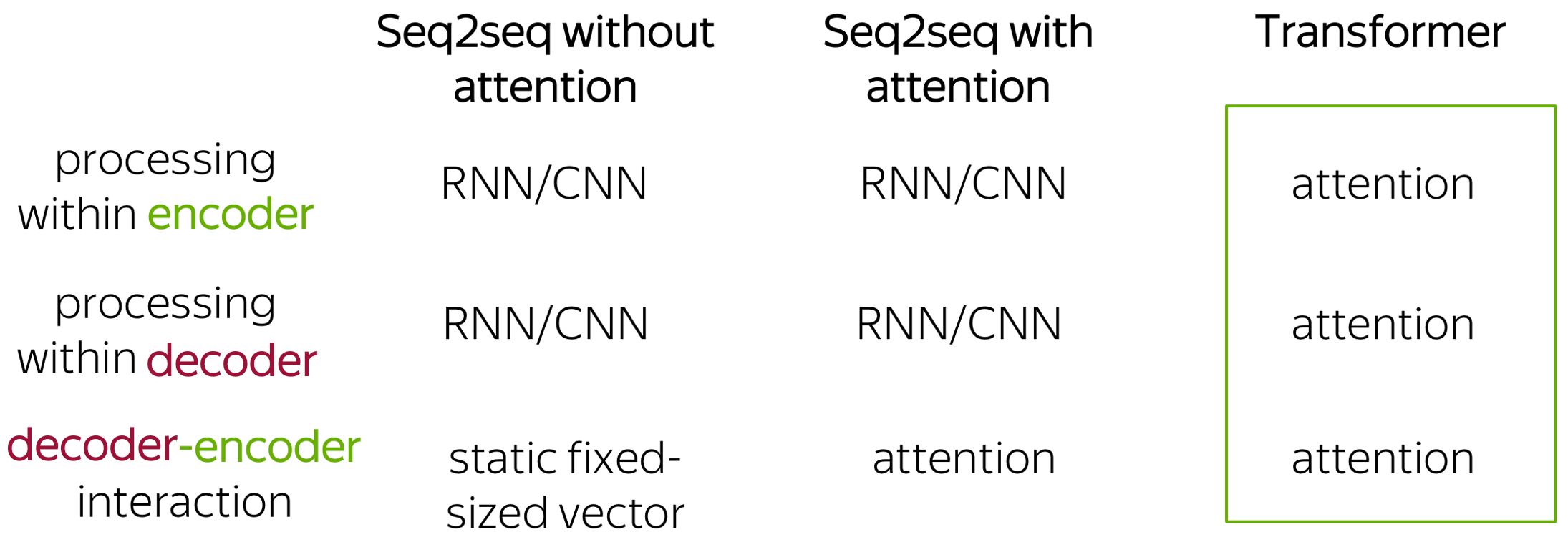
Transformer introduced a new modeling paradigm: in contrast to previous models where processing within encoder and decoder was done with recurrence or convolutions, Transformer operates using only attention.

MUST READ:

• Transformer: Attention is All You Need - Lena Voita
• Attention Attention !, Multi_head_attention
• Annotated Transformer
• How Transformers work in deep learning and NLP: an intuitive introduction

Must Watch

Why Transformer is more suitable than RNN based model?

When encoding a sentence, RNNs won’t understand what bank means until they read the whole sentence, and this can take a while for long sequences. In contrast, in Transformer’s encoder tokens interact with each other all at once.

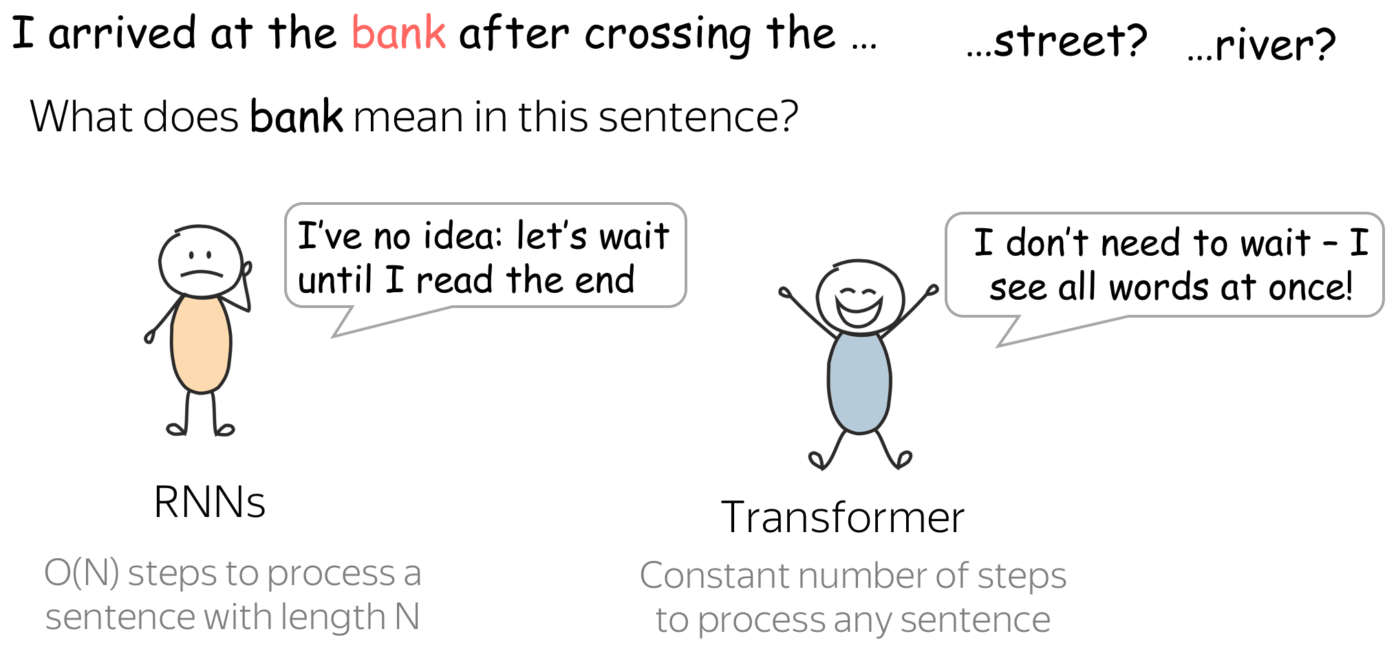
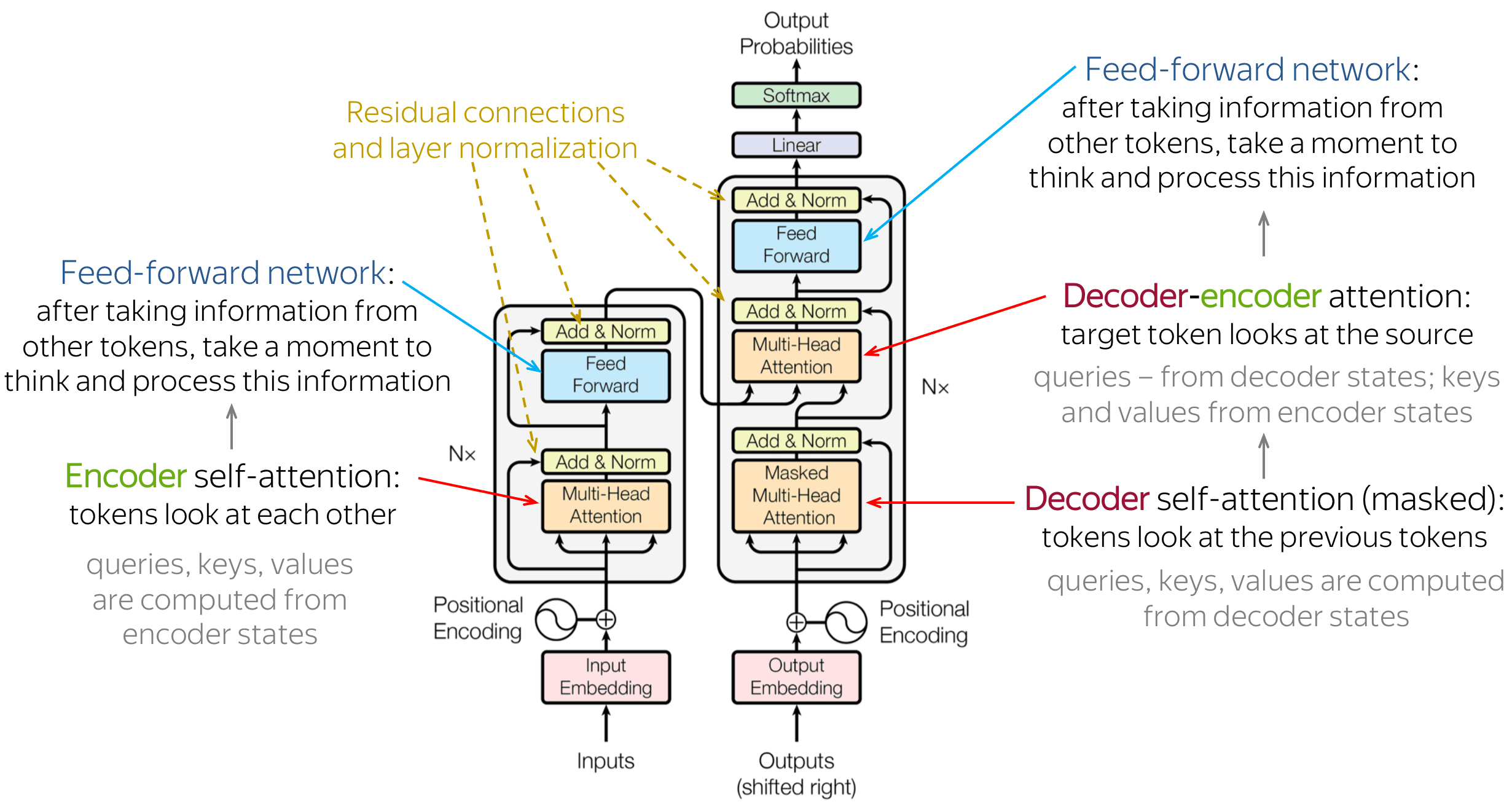
Intuitively, Transformer’s encoder can be thought of as a sequence of reasoning steps (layers). At each step, tokens look at each other (this is where we need attention - self-attention), exchange information and try to understand each other better in the context of the whole sentence. This happens in several layers.

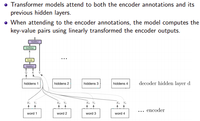
In each decoder layer, tokens of the prefix also interact with each other via a self-attention mechanism, but additionally, they look at the encoder states (without this, no translation can happen, right?).

Self-Attention: the “Look at Each Other” Part

Self-attention is one of the key components of the model. The difference between attention and self-attention is that self-attention operates between representations of the same nature: e.g., all encoder states in some layer.

There are 3 types of attention architecture

• Attention inside Encoder block (self-attention)
  • from: each state from a set of states
  • at: all other states in the same set.
• Attention inside Decoder block
  • Masked Self-Attention: “Don’t Look Ahead” for the Decoder
• Attention inside Encoder-Decoder communication
  • From: one current decoder state
  • At: all encoder states

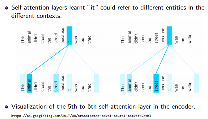
Self-attention is the part of the model where tokens interact with each other. Each token “looks” at other tokens in the sentence with an attention mechanism, gathers context, and updates the previous representation of “self”. Look at the illustration.

---

*If above link is broken, click here

• The Transformer uses attention to boost the speed with which these models can be trained.
• The biggest benefit, however, comes from how The Transformer lends itself to parallelization.
• At the core of Transformer, there is encoder-decoder block

The encoding component is a stack of encoders (the paper stacks six of them on top of each other – there’s nothing magical about the number six, one can definitely experiment with other arrangements). The decoding component is a stack of decoders of the same number.

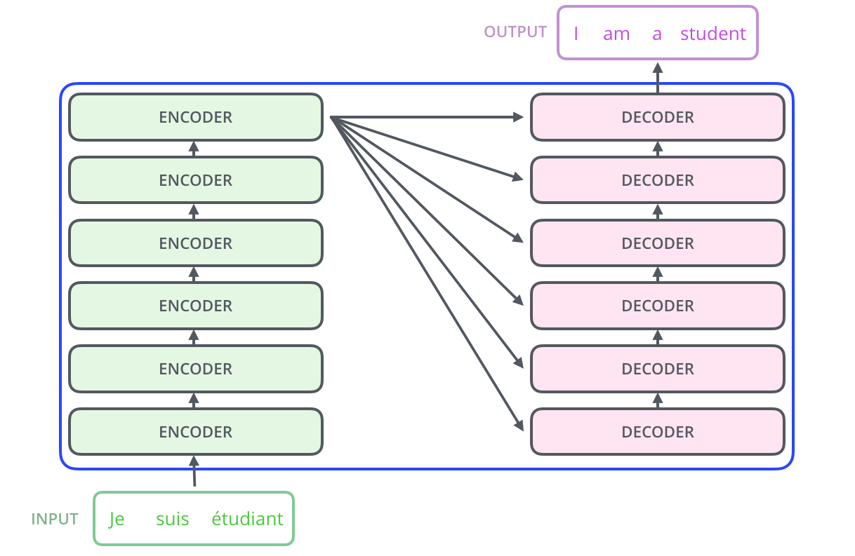
The encoders are all identical in structure (yet they do not share weights).

• Each encoder block is a combination of a FFNN and Self-Attention

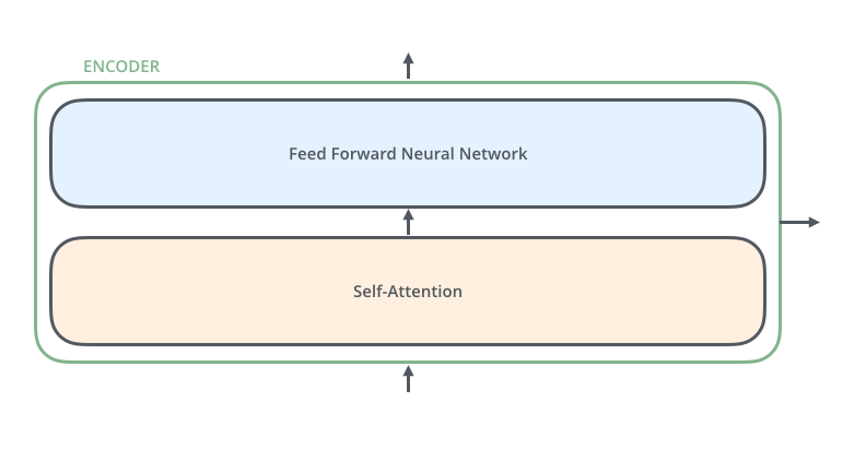
• The encoder’s inputs first flow through a self-attention layer

A layer that helps the encoder look at other words in the input sentence as it encodes a specific word.

• The FFNNs are all independent, this helps to run the code in parallel.

As multiple encoders are stacked on top of each other, ENCODER#0 receives the regular word embedding which passes through self-attention layer followed by FFNN. The output of these FFNN are form of enriched word embedding which act as input to the ENCODER#1.

The decoder has both those layers, but between them is an attention layer that helps the decoder focus on relevant parts of the input sentence

---

Self-Attention in Detail

Query, Key, and Value in Self-Attention

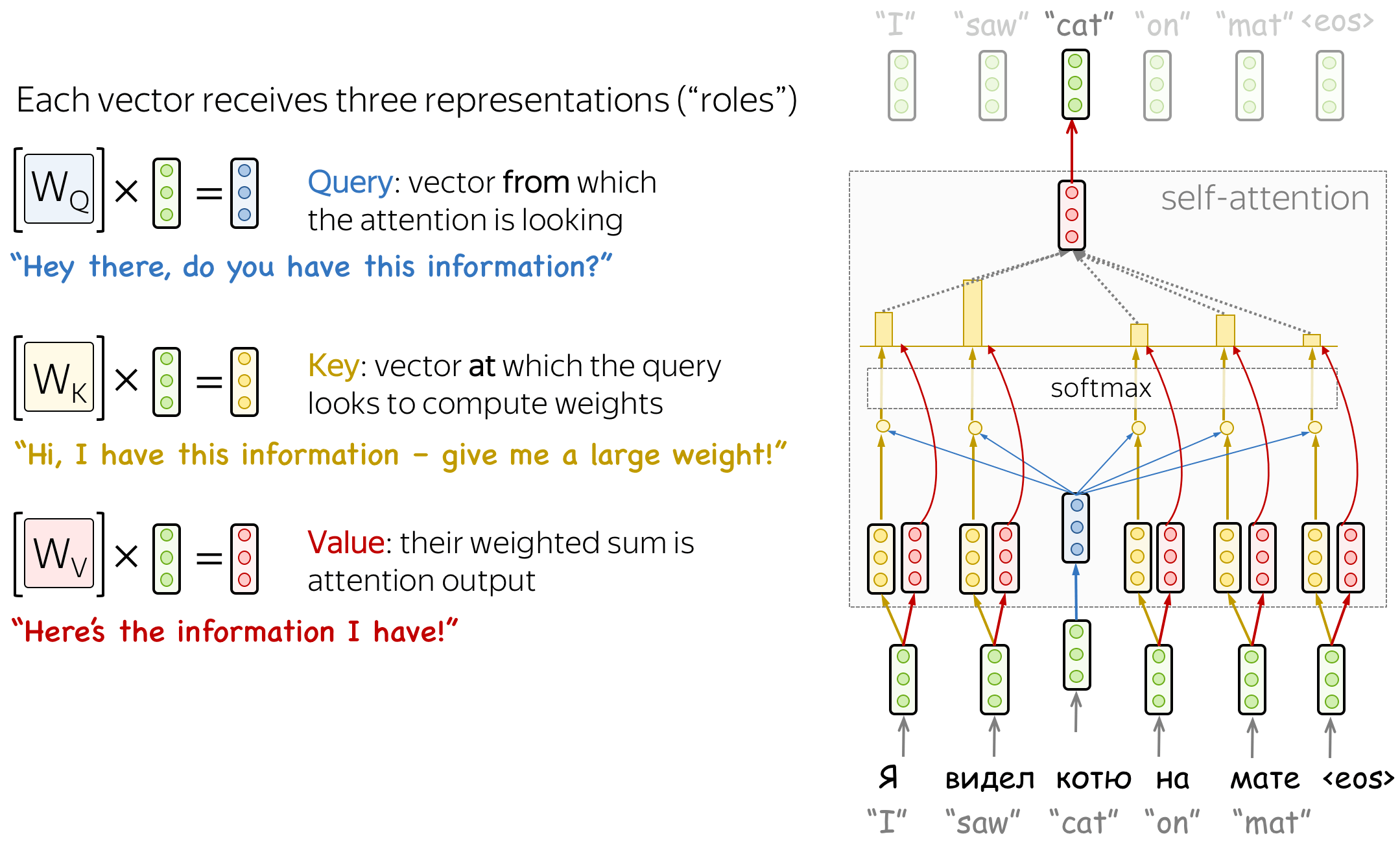
Formally, this intuition is implemented with a query-key-value attention. Each input token in self-attention receives three representations corresponding to the roles it can play:

• query - asking for information;
• key - saying that it has some information;
• value - giving the information.

The query is used when a token looks at others - it’s seeking the information to understand itself better. The key is responding to a query’s request: it is used to compute attention weights. The value is used to compute attention output: it gives information to the tokens which “say” they need it (i.e. assigned large weights to this token).

The formula for computing attention output is as follows:

*image source

Must Watch

*If above link is broken, click here

TL;DR:

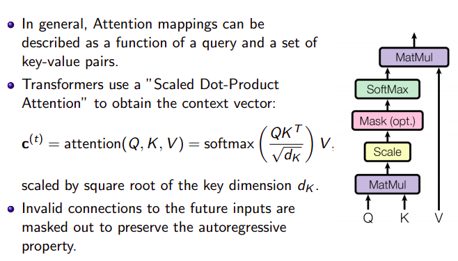
• The major component in the transformer is the unit of multi-head self-attention mechanism. The transformer views the encoded representation of the input as a set of key-value pairs, ($\mathbf{K},\mathbf{V}$), both of dimension $n$ (input sequence length); in the context of NMT, both the keys and values are the encoder hidden states. In the decoder, the previous output is compressed into a query ($\mathbf{Q}$ of dimension $m$) and the next output is produced by mapping this query and the set of keys and values.

• The transformer adopts the scaled dot-product attention: the output is a weighted sum of the values, where the weight assigned to each value is determined by the dot-product of the query with all the keys:

$ \text{Attention}(\mathbf{Q}, \mathbf{K}, \mathbf{V}) = \text{softmax}(\frac{\mathbf{Q}\mathbf{K}^\top}{\sqrt{n}})\mathbf{V} $

Details:

The first step in calculating self-attention is to create three vectors from each of the encoder’s input vectors (in this case, the embedding of each word). So for each word, we create a Query vector, a Key vector, and a Value vector. These vectors are created by multiplying the embedding by three matrices that we trained during the training process.

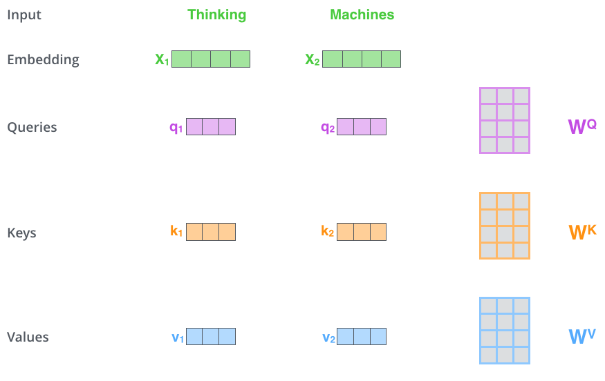
• Multiplying $x_1$ by the $W^Q$ weight matrix produces $q_1$, the query vector associated with that word. We end up creating a query, a key, and a value projection of each word in the input sentence.

What are the “query”, “key”, and “value” vectors?

• They’re abstractions that are useful for calculating and thinking about attention.

The second step in calculating self-attention is to calculate a score. Say we’re calculating the self-attention for the first word in this example, Thinking. We need to score each word of the input sentence against this word. The score determines how much focus to place on other parts of the input sentence as we encode a word at a certain position.

The third and forth steps are to divide the scores by 8 (the square root of the dimension of the key vectors used in the paper – 64. This leads to having more stable gradients and then normalize them by taking Softmax of these scores.

This softmax score determines how much each word will be expressed at this position.

The fifth step is to multiply each value vector by the softmax score (in preparation to sum them up). The intuition here is to keep intact the values of the word(s) we want to focus on, and drown-out irrelevant words (by multiplying them by tiny numbers like $0.001$, for example).

The sixth step is to sum up the weighted value vectors. This produces the output of the self-attention layer at this position (for the first word).

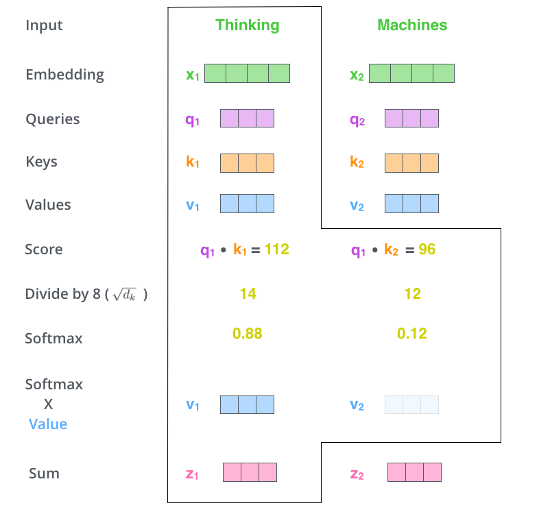
The resulting vector is one we can send along to the feed-forward neural network. In the actual implementation, however, this calculation is done in matrix form for faster processing.

Matrix Calculation of Self-Attention

The first step is to calculate the Query, Key, and Value matrices. We do that by packing our embeddings into a matrix $X$, and multiplying it by the weight matrices we’ve trained ($W^Q$, $W^K$, $W^V$).

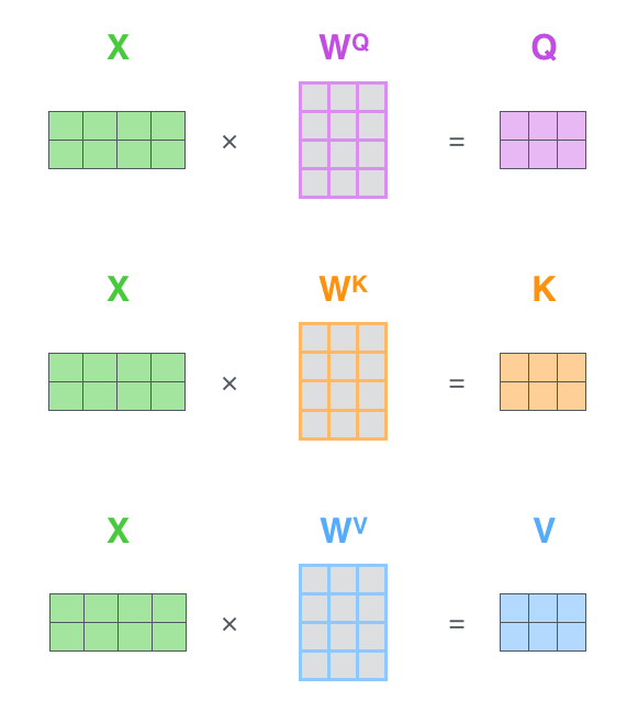
• Every row in the X matrix corresponds to a word in the input sentence.

Finally, since we’re dealing with matrices, we can condense steps two through six in one formula to calculate the outputs of the self-attention layer.

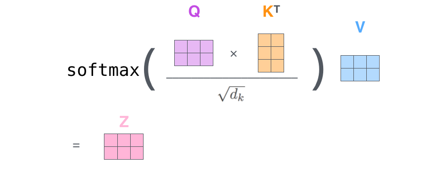
*self attention: CMU Neural Nets for NLP 2021 - Graham Neubig

---

Masked Self-Attention: “Don’t Look Ahead” for the Decoder

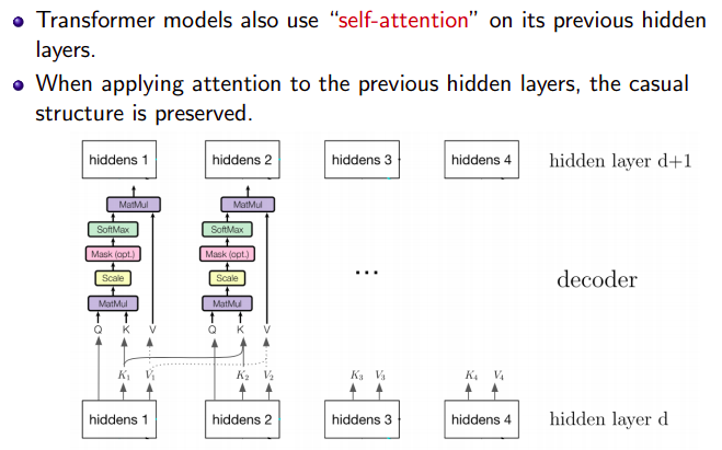
In the decoder, there’s also a self-attention mechanism: it is the one performing the “look at the previous tokens” function.

In the decoder, self-attention is a bit different from the one in the encoder. While the encoder receives all tokens at once and the tokens can look at all tokens in the input sentence, in the decoder, we generate one token at a time: during generation, we don’t know which tokens we’ll generate in future.

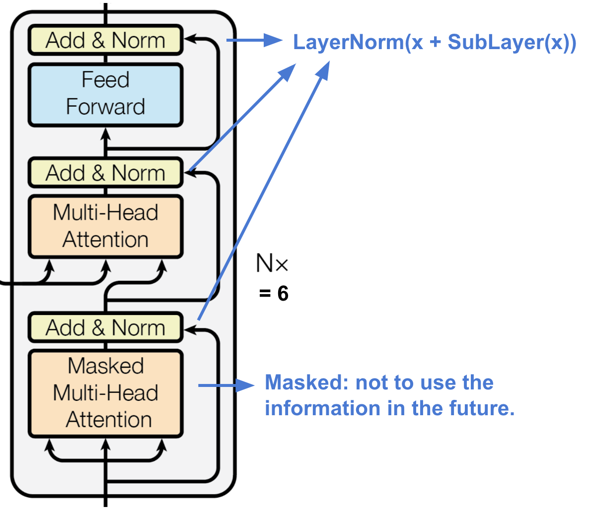
To forbid the decoder to look ahead, the model uses masked self-attention: future tokens are masked out. Look at the illustration.

But how can the decoder look ahead?

During generation, it can’t - we don’t know what comes next. But in training, we use reference translations (which we know). Therefore, in training, we feed the whole target sentence to the decoder - without masks, the tokens would “see future”, and this is not what we want.

This is done for computational efficiency: the Transformer does not have a recurrence, so all tokens can be processed at once. This is one of the reasons it has become so popular for machine translation - it’s much faster to train than the once dominant recurrent models. For recurrent models, one training step requires O(len(source) + len(target)) steps, but for Transformer, it’s O(1), i.e. constant.

Multi Headed Attention: Independently Focus on Different Things

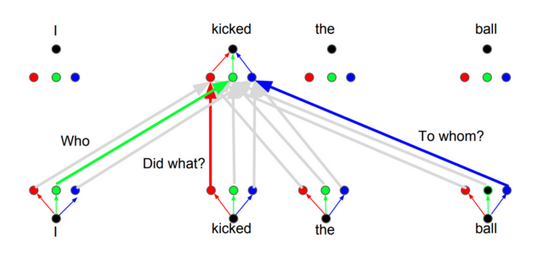
The idea behind it is that whenever you are translating a word, you may pay different attention to each word based on the type of queries that you are asking. The images below show what that means.

Input: Bob kicked the ball.

• Query 1: Who kicked? $\rightarrow$ Value 1: Bob
• Query 2: What kicked? $\rightarrow$ Value 2: Ball
• Query 3: Did what? $\rightarrow$ Value 3: Kicked

Depending on the answer, the translation of the word to another language can change. Or ask other questions. [pay attention to this, for Multi Head Attention later]

must read: slide, blog

Must Watch

*If above link is broken, click here

TL;DR:

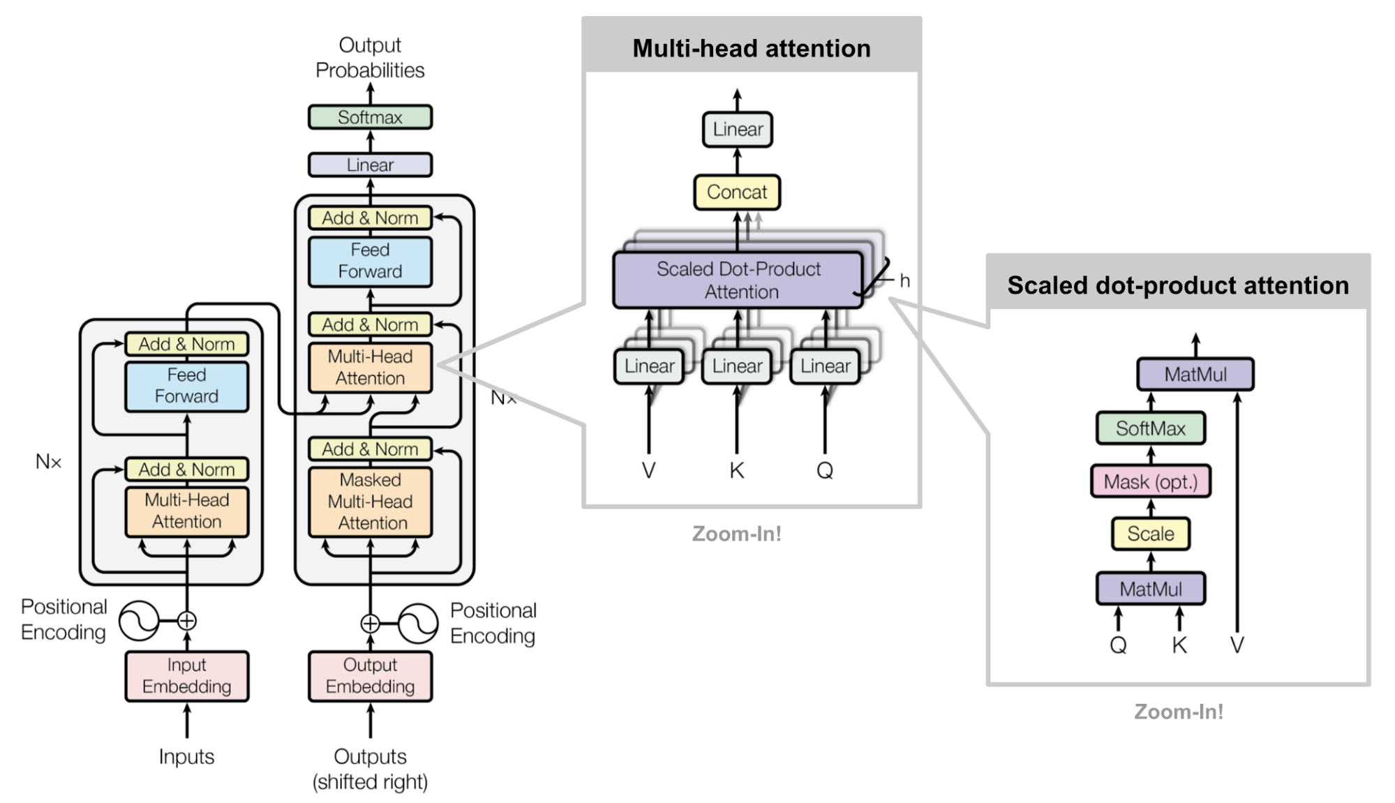
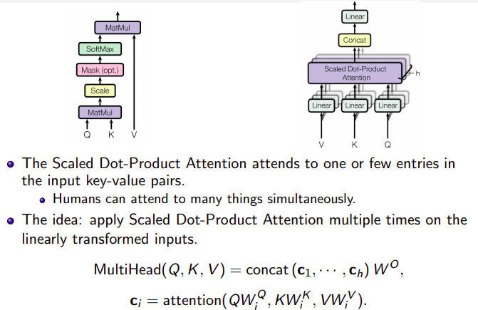
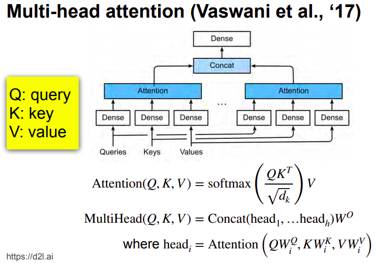
Rather than only computing the attention once, the multi-head mechanism runs through the scaled dot-product attention multiple times in parallel.

The independent attention outputs are simply concatenated and linearly transformed into the expected dimensions. I assume the motivation is because ensembling always helps? ;) According to the paper, “multi-head attention allows the model to jointly attend to information from different representation subspaces at different positions. With a single attention head, averaging inhibits this.”

$ \text{MultiHead}(\mathbf{Q}, \mathbf{K}, \mathbf{V}) = [\text{head}_1; \dots; \text{head}_h]\mathbf{W}^O $ $ \text{where head}_i = \text{Attention}(\mathbf{Q}\mathbf{W}^Q_i, \mathbf{K}\mathbf{W}^K_i, \mathbf{V}\mathbf{W}^V_i) $

where $\mathbf{W}^Q_i$, $\mathbf{W}^K_i$ , $\mathbf{W}^V_i$, and $\mathbf{W}^O$ are parameter matrices to be learned.

Usually, understanding the role of a word in a sentence requires understanding how it is related to different parts of the sentence. This is important not only in processing source sentence but also in generating target. For example, in some languages, subjects define verb inflection (e.g., gender agreement), verbs define the case of their objects, and many more. What I’m trying to say is: each word is part of many relations.

Therefore, we have to let the model focus on different things: this is the motivation behind Multi-Head Attention. Instead of having one attention mechanism, multi-head attention has several “heads” which work independently.

Formally, this is implemented as several attention mechanisms whose results are combined:

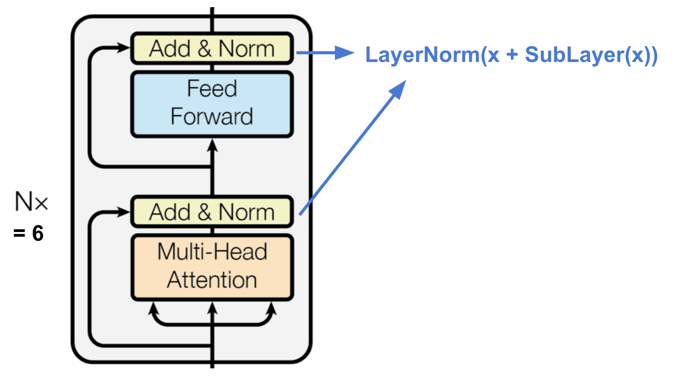
ENCODER:

DECODER:

FULL ARCHITECTURE

MUST READ

Details:

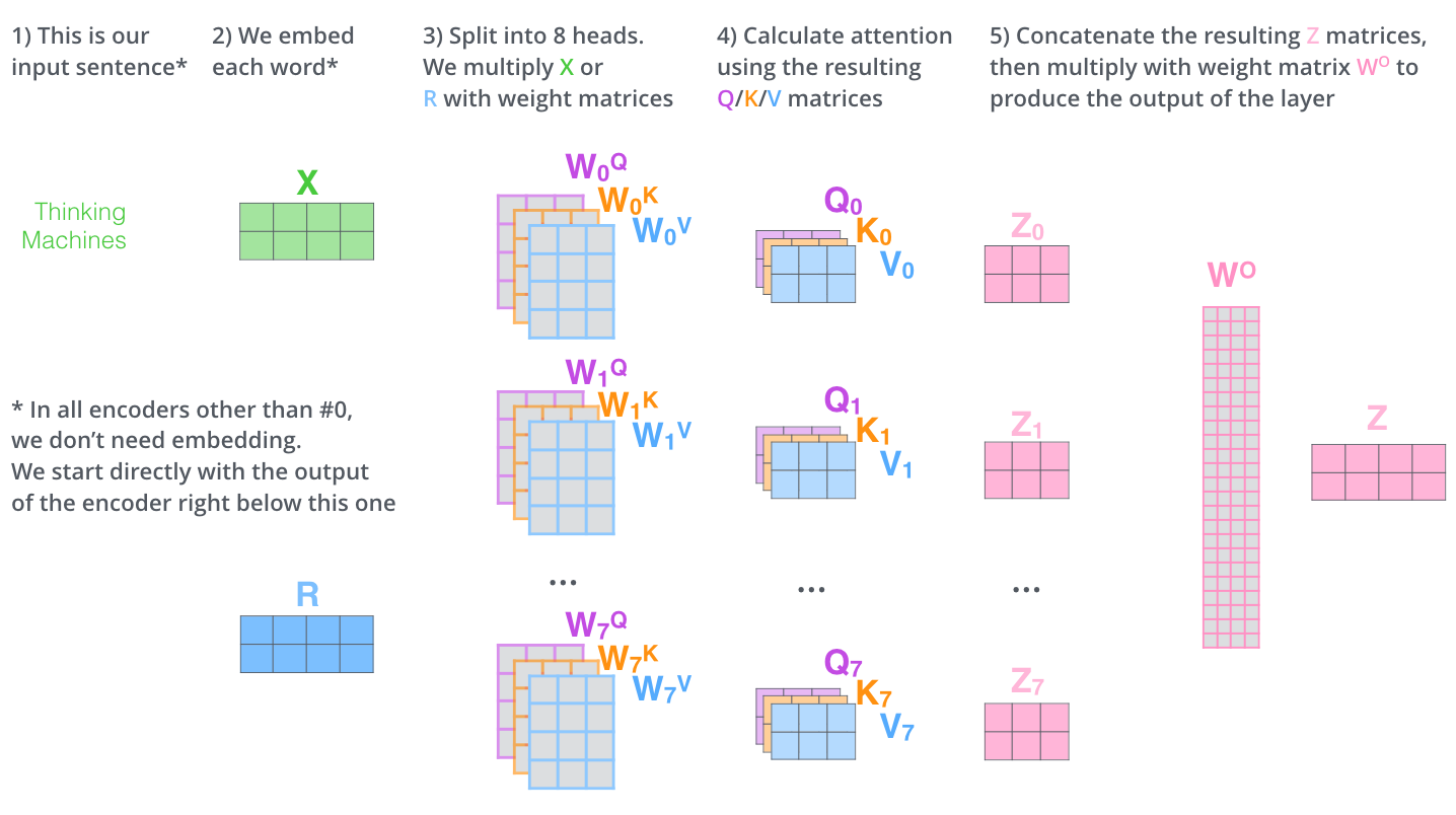
The paper further refined the self-attention layer by adding a mechanism called “multi-headed” attention. This improves the performance of the attention layer in two ways:

1. It expands the model’s ability to focus on different positions. In the example above, $z_1$ contains a little bit of every other encoding, but it could be dominated by the the actual word itself.
2. It gives the attention layer multiple representation subspaces.
   1. With multi-headed attention, we maintain separate $Q_i/K_i/V_i$ weight matrices for each head resulting in different $Q_i/K_i/V_i$ matrices. As we did before, we multiply $X$ by the $W_i^Q/W_i^K/W_i^V$ matrices to produce $Q/K/V$ matrices. Here $i$ represents the $i^{th}$ head.
   2. In the original paper they used $8$ heads.

Multiple Head is asking as if multiple queries to the same sentence, to highlight (attend) multiple values (words/tokens).

All the different heads give different $z_i$ matrices. Concat them and multiply with weight matrix $W^O$ (trained jointly with the model) to get the final $z$ matrix that captures information from all the attention heads. This final $z$ can be sent to the FFNN.

Summarizing all here it is:

Positional Encoding

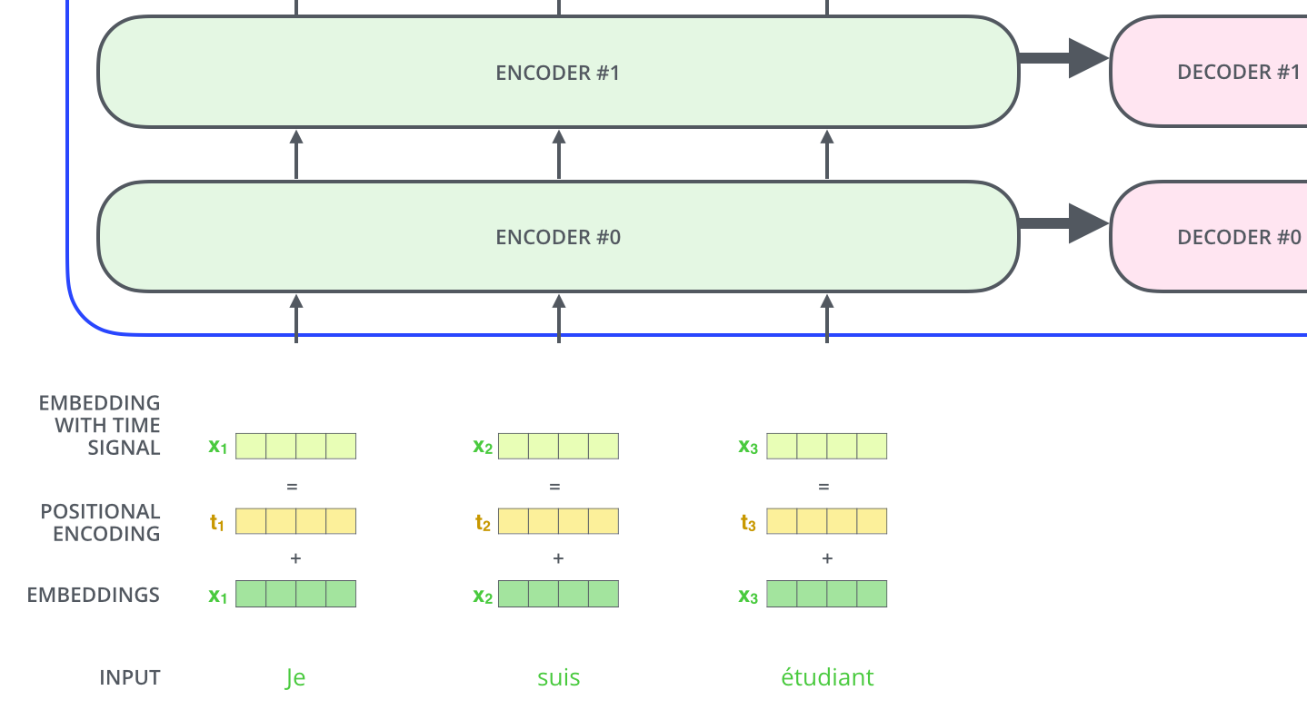
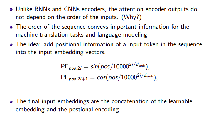
One thing that’s missing from the model as we have described it so far is a way to account for the order of the words in the input sequence.

To address this, the transformer adds a vector to each input embedding. These positional encoding vectors are also learnt. These vectors follow a specific pattern that the model learns, which helps it determine the position of each word, or the distance between different words in the sequence.

The Residuals

One detail in the architecture of the encoder that we need to mention before moving on, is that each sub-layer (self-attention, ffnn) in each encoder has a residual connection around it, and is followed by a layer-normalization step.

If we’re to visualize the vectors and the layer-norm operation associated with self attention, it would look like this:

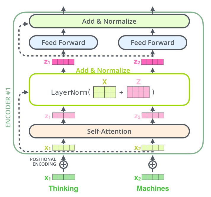
This goes for the sub-layers of the decoder as well. If we’re to think of a Transformer of 2 stacked encoders and decoders, it would look something like this:

The Decoder Side

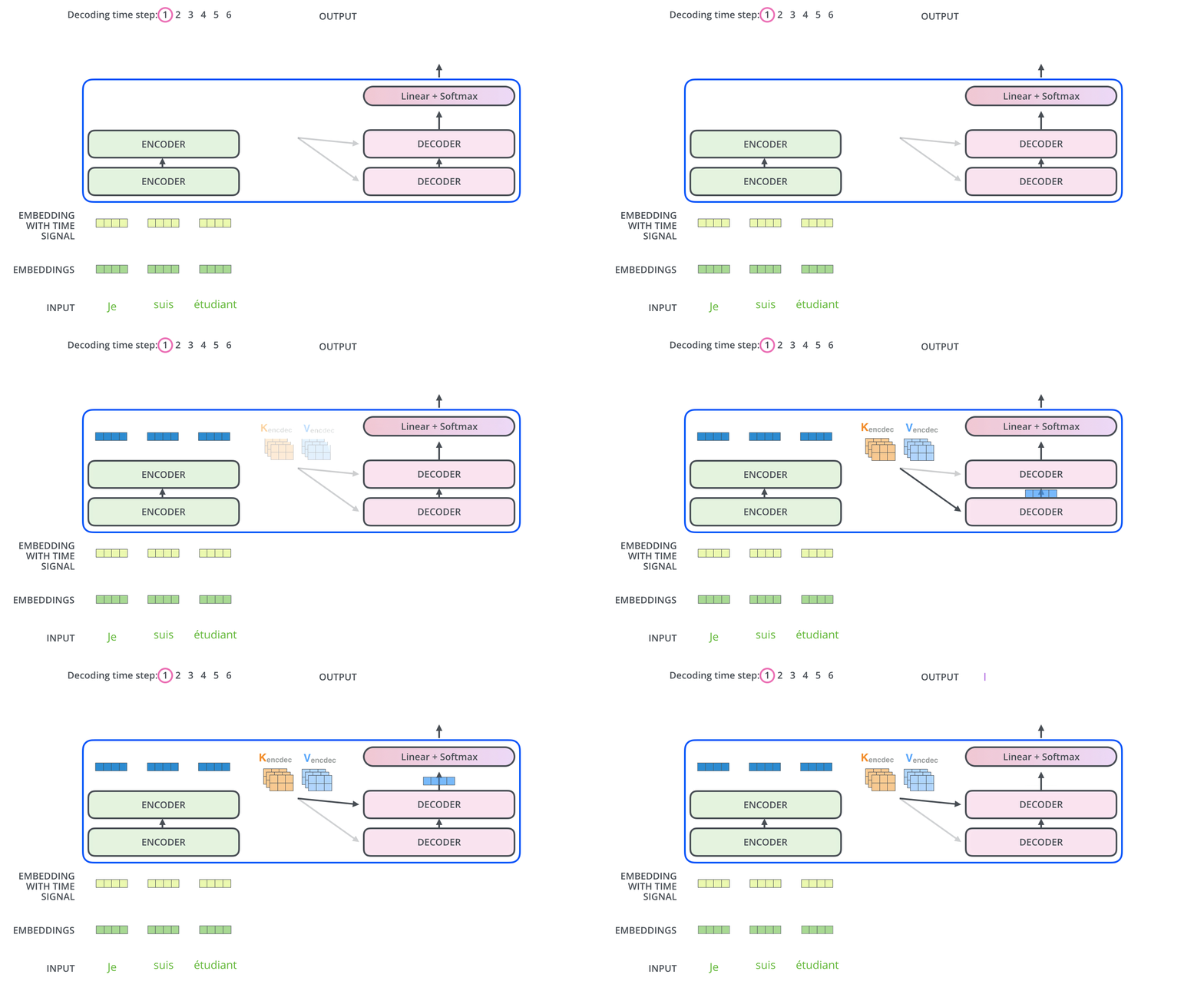
Now that we’ve covered most of the concepts on the encoder side, we basically know how the components of decoders work as well. But let’s take a look at how they work together.

Reference:

• The Illustrated Transformer by Jay Alammar
• The Annotated Transformer
• How Transformers Work

---

Transformer - Deeper Understanding

The following content has been borrowed from D2L: Alex Smola, Transformer for educational purpose.

Let’s recap the pros and cons of CNN and RNN:

• CNNs are easy to parallelize at a layer but cannot capture the variable-length sequential dependency very well.
• RNNs are able to capture the long-range, variable-length sequential information, but suffer from inability to parallelize within a sequence.

To combine the advantages from both CNNs and RNNs, Vaswani et al., 2017 designed a novel architecture using the attention mechanism. This architecture, which is called as Transformer, achieves

1. Parallelization by capturing recurrence sequence with attention
2. At the same time encodes each item’s position in the sequence.

As a result, Transformer leads to a compatible model with significantly shorter training time.

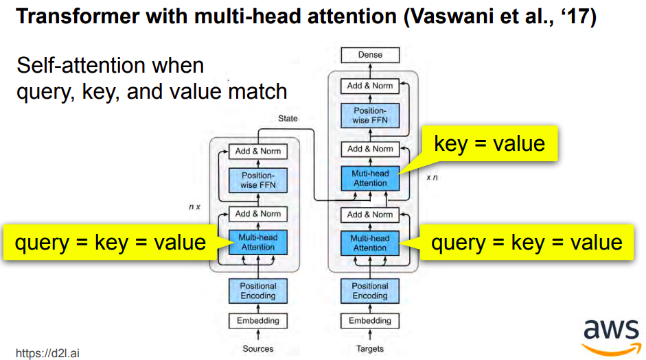
Similar to the seq2seq model, Transformer is also based on the encoder-decoder architecture. However, Transformer differs to the former as follows:

Salient features of transformers:

1. Replacing the recurrent layers in seq2seq with multi-head attention layers
2. Incorporating the position-wise information through position encoding
3. Applying layer normalization.

---

Comapre Transformer with Seq2Seq model

We compare Transformer and seq2seq side-by-side in the below figure

Similarity:

• The source sequence embeddings are fed into $n$ repeated blocks. The outputs of the last block are then used as attention memory for the decoder.
• The target sequence embeddings are similarly fed into $n$ repeated blocks in the decoder, and the final outputs are obtained by applying a dense layer with vocabulary size to the last block’s outputs.

Dissimilarity

• Transformer block: a recurrent layer in seq2seq is replaced by a Transformer block. This block contains
  • a multi-head attention layer
  • a network with two position-wise feed-forward network layers for the encoder.
  • For the decoder, another multi-head attention layer is used to take the encoder state.
• Add and norm: the inputs and outputs of both the multi-head attention layer or the position-wise feed-forward network, are processed by two add and norm layer that contains a residual structure and a layer normalization layer.
• Position encoding: Since the self-attention layer does not distinguish the item order in a sequence, a positional encoding layer is used to add sequential information into each sequence item.

---

Multi-Head Attention

Before the discussion of the multi-head attention layer, let’s quick express the self-attention architecture. The self-attention model is a normal attention model, with its query, its key, and its value being copied exactly the same from each item of the sequential inputs. As we illustrate in the below figure, self-attention outputs a same-length sequential output for each input item. Compared with a recurrent layer, output items of a self-attention layer can be computed in parallel and, therefore, it is easy to obtain a highly-efficient implementation.

The multi-head attention layer consists of $h$ parallel self-attention layers, each one is called a head. For each head, before feeding into the attention layer, we project the queries, keys, and values with three dense layers with hidden sizes $p_q$, $p_k$, and $p_v$, respectively. The outputs of these $h$ attention heads are concatenated and then processed by a final dense layer.

Assume that the dimension for a query, a key, and a value are $d_q$, $d_k$, and $d_v$, respectively. Then, for each head $i=1, \dots ,h$, we can train learnable parameters $W^{(i)}_q \in \mathbb{R}^{p_q \times d_q}$, $W^{(i)}_k \in \mathbb{R}^{p_k \times d_k}$ , and $W^{(i)}_v \in \mathbb{R}^{p_v \times d_v}$. Therefore, the output for each head is

$ o^{(i)} = attention(W^{(i)}_q q,W^{(i)}_k k, W^{(i)}_v v ) $

where attention can be any attention layer, such as the DotProductAttention and MLPAttention.

After that, the output with length $p_v$ from each of the $h$ attention heads are concatenated to be an output of length $h p_v$, which is then passed the final dense layer with $d_o$ hidden units. The weights of this dense layer can be denoted by $W_o \in \mathbf{R}^{d_o \times hp_v}$. As a result, the multi-head attention output will be

$ \mathbf o = \mathbf W_o \begin{bmatrix} \mathbf o^{(1)}\\\vdots\\\mathbf o^{(h)} \end{bmatrix} $

Multi-Head Self-Attention: What are these heads doing?

First, let’s start with our traditional model analysis method: looking at model components. Previously, we looked at convolutional filters in classifiers, neurons in language models; now, it’s time to look at a bigger component: attention. But let’s take not the vanilla one, but the heads in Transformer’s multi-head attention.

First, why are we doing this? Multi-head attention is an inductive bias (is the set of assumptions that the learner uses to predict outputs of given inputs that it has not encountered) introduced in the Transformer. When creating an inductive bias in a model, we usually have some kind of intuition for why we think this new model component, inductive bias, could be useful. Therefore, it’s good to understand how this new thing works - does it learn the things we thought it would? If not, why it helps? If yes, how can we improve it? Hope now you are motivated enough, so let’s continue.

The Most Important Heads are Interpretable

Here we’ll mention some of the results from the ACL 2019 paper Analyzing Multi-Head Self-Attention: Specialized Heads Do the Heavy Lifting, the Rest Can Be Pruned. The authors look at individual attention heads in encoder’s multi-head attention and evaluate how much, on average, different heads “contribute” to generated translations (for the details on how exactly they did this, look in the paper or the blog post ). As it turns out,

Only a small number of heads are important for translation, these heads play interpretable “roles”. These roles are:

• positional: attend to a token’s immediate neighbors, and the model has several such heads (usually 2-3 heads looking at the previous token and 2 heads looking at the next token);
• syntactic: learned to track some major syntactic relations in the sentence (subject-verb, verb-object);
• rare tokens: the most important head on the first layer attends to the least frequent tokens in a sentence (this is true for models trained on different language pairs!).

Reference:

• Analysis and Interpretability of heads - Lena Voita

---

Position-wise Feed-Forward Networks

• Another key component in the Transformer block is called position-wise feed-forward network (FFN). It accepts a $3$-dimensional input with shape (batch size, sequence length, feature size).
• The position-wise FFN consists of two dense layers that applies to the last dimension. Since the same two dense layers are used for each position item in the sequence, we referred to it as position-wise. Indeed, it is equivalent to applying two $1 \times 1$ convolution layers.

Add and Norm

Besides the above two components in the Transformer block, the add and norm within the block also plays a key role to connect the inputs and outputs of other layers smoothly. To explain, we add a layer that contains a residual structure and a layer normalization after both the multi-head attention layer and the position-wise FFN network.

Layer normalization is similar to batch normalization. One difference is that the mean and variances for the layer normalization are calculated along the last dimension, e.g X.mean(axis=-1) instead of the first batch dimension, e.g., X.mean(axis=0).

Layer normalization prevents the range of values in the layers from changing too much, which means that faster training and better generalization ability.

Positional Encoding

Unlike the recurrent layer, both the multi-head attention layer and the position-wise feed-forward network compute the output of each item in the sequence independently. This feature enables us to parallelize the computation, but it fails to model the sequential information for a given sequence.

To better capture the sequential information, the Transformer model uses the positional encoding to maintain the positional information of the input sequence.

To explain, assume that $X \in \mathbb{R}^{l×d}$ is the embedding of an example, where $l$ is the sequence length and $d$ is the embedding size. This positional encoding layer encodes $X$’s position $P \in \mathbb{R}^{l \times d}$ and outputs $P+X$.

The position $P$ is a $2$-D matrix, where

• $i$ refers to the order in the sentence
• $j$ refers to the position along the embedding vector dimension.

In this way, each value in the original sequence is then maintained using the equations below:

$ P_{i, 2j} = \sin(i/10000^{2j/d}) $ $ P_{i, 2j+1} = \cos(i/10000^{2j/d}) $

for $i=0,\ldots, l-1$ and $j=0,\ldots,\lfloor(d-1)/2\rfloor$.

Why do we need it in the first place?

Transformer architecture ditched the recurrence mechanism in favor of multi-head self-attention mechanism. Avoiding the RNNs’ method of recurrence will result in massive speed-up in the training time. And theoretically, it can capture longer dependencies in a sentence.

The model itself doesn’t have any sense of position/order for each word. Consequently, there’s still the need for a way to incorporate the order of the words into our model. One possible solution to give the model some sense of order is to add a piece of information to each word about its position in the sentence. We call this “piece of information”, the positional encoding.

Ideally, the following criteria should be satisfied:

• Unique Positional Encoding It should output a unique encoding for each time-step (word’s position in a sentence)
• Consistent Distance: Distance between any two time-steps should be consistent across sentences with different lengths.
• Model should generalize to longer sentences without any efforts. Its values should be bounded.
• It must be deterministic.

Intuition of $\sin$ and $\cos$ in positional encoding:

A more intuitive explanation of positional embedding is to think about it as a clock (as cos and sin are just concept from unit circle). Every two dimension of the positional embedding just specifies one of the clock’s hand (the hour hand, the minute hand, the second hand, for example). Then moving from one position to the next position is just rotating those hands at different frequencies. Thus, without formal proof, it immediately tells you why a rotation matrix exist.

Reference:

• Transformer Architecture: The Positional Encoding [read comment section]
• proof

---

What is position wise FFN?

From the author of “Attention is all you need” by Vaswani et al.

In addition to attention sub-layers, each of the layers in our encoder and decoder contains a fully connected feed-forward network, which is applied to each position separately and identically. This consists of two linear transformations with a ReLU activation in between.

$ FFN(𝑥)=max(0,𝑥×𝑊_1+𝑏_1)×𝑊_2+𝑏_2 $

While the linear transformations are the same across different positions, they use different parameters from layer to layer. Another way of describing this is as two convolutions with kernel size 1. The dimensionality of input and output is $𝑑_{model}=512$, and the inner-layer has dimensionality $𝑑_{𝑓𝑓}=2048$.

Reference:

• stackexchange

---

Encoder

Armed with all the essential components of Transformer, let’s first build a Transformer encoder block. This encoder contains a

1. Multi-head attention layer
2. A position-wise feed-forward network
3. Two add and norm connection blocks.

As shown in the code (section 10.3.5), for both of the attention model and the positional FFN model in the EncoderBlock, their outputs’ dimension are equal to the num_hiddens.

This is due to the nature of the residual block, as we need to add these outputs back to the original value during add and norm.

Decoder

The Transformer decoder block looks similar to the Transformer encoder block. However, besides the two sub-layers (1. the multi-head attention layer and 2. the positional encoding network), the decoder Transformer block contains a third sub-layer, which applies multi-head attention on the output of the encoder stack.

Similar to the Transformer encoder block, the Transformer decoder block employs add and norm, i.e., the residual connections and the layer normalization to connect each of the sub-layers.

To be specific, at time-step $t$, assume that $x_t$ is the current input, i.e., the query. As illustrated in the below figure, the keys and values of the self-attention layer consist of the current query with all the past queries $x_1 \ldots ,x_{t−1}$.

During training, the output for the $t$-query could observe all the previous key-value pairs. It results in an different behavior from prediction. Thus, during prediction we can eliminate the unnecessary information by specifying the valid length to be $t$ for the $t^{th}$ query.

Reference:

• D2L: Alex Smola, Transformer
• IMP: The Annotated Transformer

---

Subword Segmentation: Byte Pair Encoding

Dealing with rare words

Character level embeddings aside, the first real breakthrough at addressing the rare words problem was made by the researchers at the University of Edinburgh by applying subword units in Neural Machine Translation using Byte Pair Encoding (BPE). Today, subword tokenization schemes inspired by BPE have become the norm in most advanced models including the very popular family of contextual language models like BERT, GPT-2, RoBERTa, etc.

The Origins of Byte Pair Encoding

Like many other applications of deep learning being inspired by traditional science, Byte Pair Encoding (BPE) subword tokenization also finds its roots deep within a simple lossless data compression algorithm. BPE was first introduced by Philip Gage in the article “A New Algorithm for Data Compression” in the February 1994 edition of the C Users Journal as a technique for data compression that works by replacing common pairs of consecutive bytes with a byte that does not appear in that data.

Repurposing BPE for Subword Tokenization

As we know, a model has a predefined vocabulary of tokens. Those input tokens, which are not in the vocabulary, will be replaced with a special UNK (“unknown”) token. Therefore, if you use the straightforward word-level tokenization (i.e., your tokens are words), you will be able to process a fixed number of words. This is the fixed vocabulary problem : you will be getting lot’s of unknown tokens, and your model won’t translate them properly.

But how can we represent all words, even those we haven’t seen in the training data?

Well, even if you are not familiar with a word, you are familiar with the parts it consists of - subwords (in the worst case, symbols).

Then why don’t we split the rare and unknown words into smaller parts? This is exactly what was proposed in the paper Neural Machine Translation of Rare Words with Subword Units by Rico Sennrich, Barry Haddow and Alexandra Birch. They introduced the de-facto standard subword segmentation, Byte Pair Encoding (BPE). BPE keeps frequent words intact and splits rare and unknown ones into smaller known parts.

What we refer to as BPE now is an adaptation of this algorithm for word segmentation. Instead of merging frequent pairs of bytes, it merges characters or character sequences.

BPE algorithm consists of two parts:

• training - learn “BPE rules”, i.e., which pairs of symbols to merge;
• inference - apply learned rules to segment a text.

Training: learn BPE rules

At this step, the algorithm builds a merge table and a vocabulary of tokens. The initial vocabulary consists of characters and an empty merge table. At this step, each word is segmented as a sequence if characters. After that, the algorithm is as follows:

• count pairs of symbols: how many times each pair occurs together in the training data;
• find the most frequent pair of symbols;
• merge this pair - add a merge to the merge table, and the new token to the vocabulary.

In practice, the algorithm first counts how many times each word appeared in the data. Using this information, it can count pairs of symbols more easily. Note also that the tokens do not cross word boundary - everything happens within words.

Look at the illustration. Here I show you a toy example: here we assume that in training data, we met cat 4 times, mat 5 times and mats, mate, ate, eat 2, 3, 3, 2 times, respectively. We also have to set the maximum number of merges we want; usually, it’s going to be about 4k-32k depending on the dataset size, but for our toy example, let’s set it to 5.

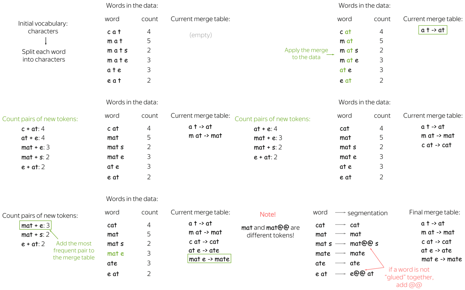
When we reached the maximum number of merges, not all words were merged into a single token. For example, mats is segmented as two tokens: mat@@ s. Note that after segmentation, we add the special characters @@ to distinguish between tokens that represent entire words and tokens that represent parts of words. In our example, mat and mat@@ are different tokens.

Implementation note: In an implementation, you need to make sure that a new merge adds only one new token to the vocabulary. For this, you can either add a special end-of-word symbol to each word (as done in the original BPE paper) or replace spaces with a special symbol (as done in e.g. Sentencepiece and YouTokenToMe, the fastest implementation), or do something else. In the illustration, I omit this for simplicity.

Inference: segment a text

After learning BPE rules, you have a merge table - now, we will use it to segment a new text.

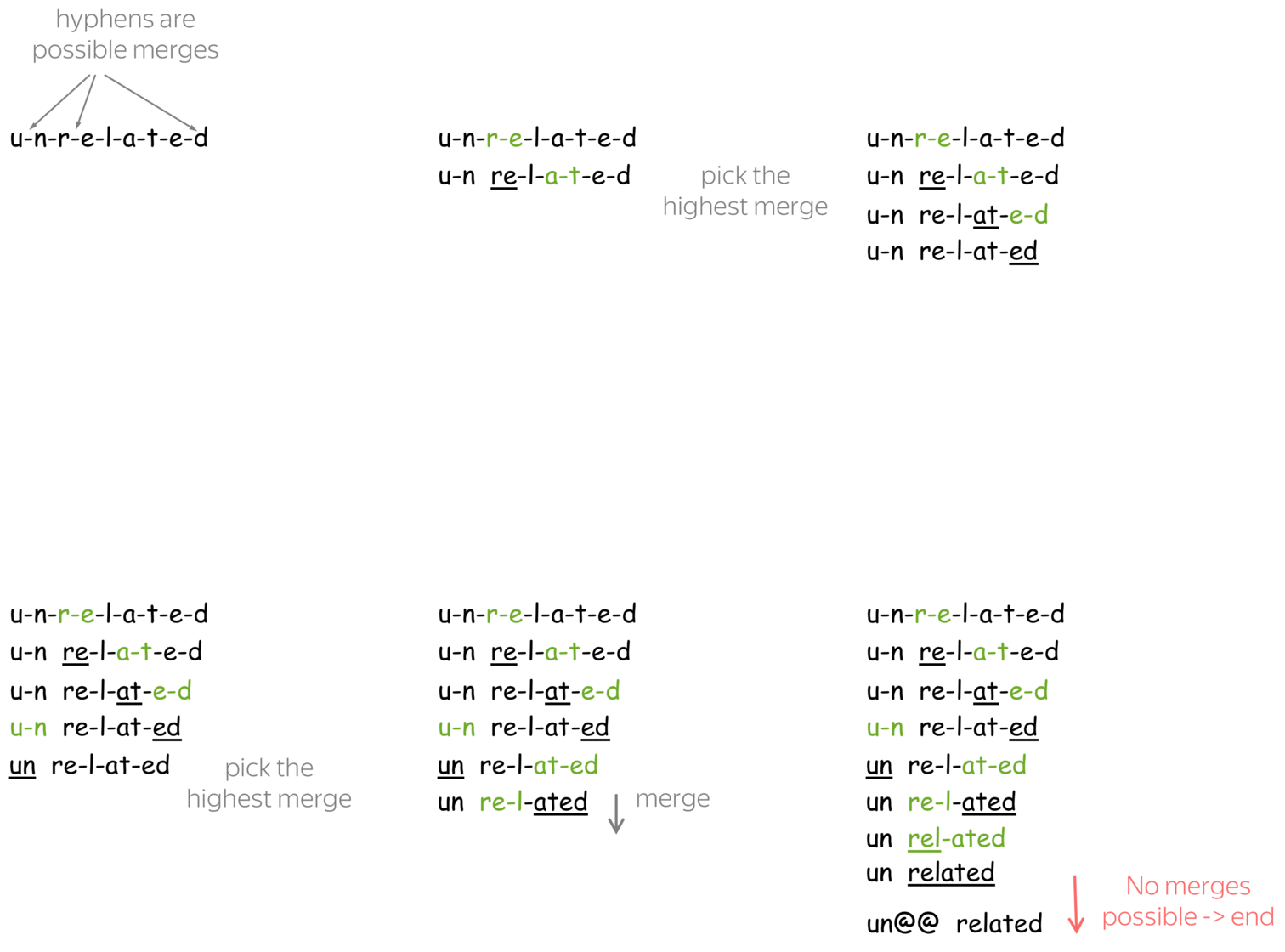
The algorithm starts with segmenting a word into a sequence of characters. After that, it iteratively makes the following two steps until no merge it possible:

• Among all possible merges at this step, find the highest merge in the table;
• Apply this merge.

Note that the merge table is ordered - the merges that are higher in the table were more frequent in the data. That’s why in the algorithm, merges that are higher have higher priority: at each step, we merge the most frequent merge among all possible.

What makes BPE the secret sauce?

BPE brings the perfect balance between character- and word-level hybrid representations which makes it capable of managing large corpora. This behavior also enables the encoding of any rare words in the vocabulary with appropriate subword tokens without introducing any “unknown” tokens. This especially applies to foreign languages like German where the presence of many compound words can make it hard to learn a rich vocabulary otherwise. With this tokenization algorithm, every word can now overcome their fear of being forgotten (athazagoraphobia).

Reference:

• Transformer - Lena Voita
• Byte Pair Encoding — The Dark Horse of Modern NLP

---

How does Attention Work ?

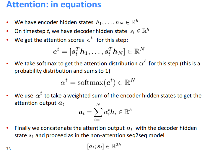
• At each time step we come up with a distribution on the input words.

• In the above image at time $t_3$, input ja raha gets the attention and it’s corresponding distributoin is $[0,0,0.5, 0.5, 0]$. This helps in modelling because now input jaa raha is linked to output going with more attention as in the attention vector other words got $0$.
• This distribution tells us how much attention to pay to some part of the input but not all parts.
• At each time step we should feed this relevant information (i.e. encoding of relevant words in the form of attention distribution) to the decoder.

In reality this distribution is not available beforehand and is learnt through the model.

[reference: Prof. Mikesh, Padhai Lecture, Encoder-Decoder]

The attention-mechanism looks at an input sequence and decides at each step which other parts of the sequence are important.

When reading a text, you always focus on the word you read but at the same time your mind still holds the important keywords of the text in memory in order to provide context.

An attention-mechanism works similarly for a given sequence. For our example with the human Encoder and Decoder, imagine that instead of only writing down the translation of the sentence in the imaginary language, the Encoder also writes down keywords that are important to the semantics of the sentence, and gives them to the Decoder in addition to the regular translation. Those new keywords make the translation much easier for the Decoder because it knows what parts of the sentence are important and which key terms give the sentence context.

Attention

The basic idea: each time the model predicts an output word, it only uses parts of an input where the most relevant information is concentrated instead of an entire sentence. In other words, it only pays attention to some input words. Let’s investigate how this is implemented.

An illustration of the attention mechanism (RNNSearch) proposed by [Bahdanau, 2014]. Instead of converting the entire input sequence into a single context vector, we create a separate context vector for each output (target) word. These vectors consist of the weighted sums of encoder’s hidden states.

Encoder works as usual, and the difference is only on the decoder’s part. As you can see from a picture, the decoder’s hidden state is computed with a context vector, the previous output and the previous hidden state. But now we use not a single context vector $c$, but a separate context vector $c_i$ for each target word.

References:

• Paper: Effective Approaches to Attention-based Neural Machine Translation
• Visualizing A Neural Machine Translation Model by Jay Alammar
• Important Blog
• Imp: Attention in NLP
• Imp: Attention and Memory in NLP

---

Encoder-Decoder with Attention

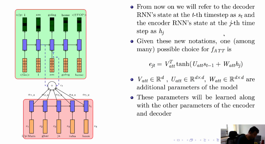
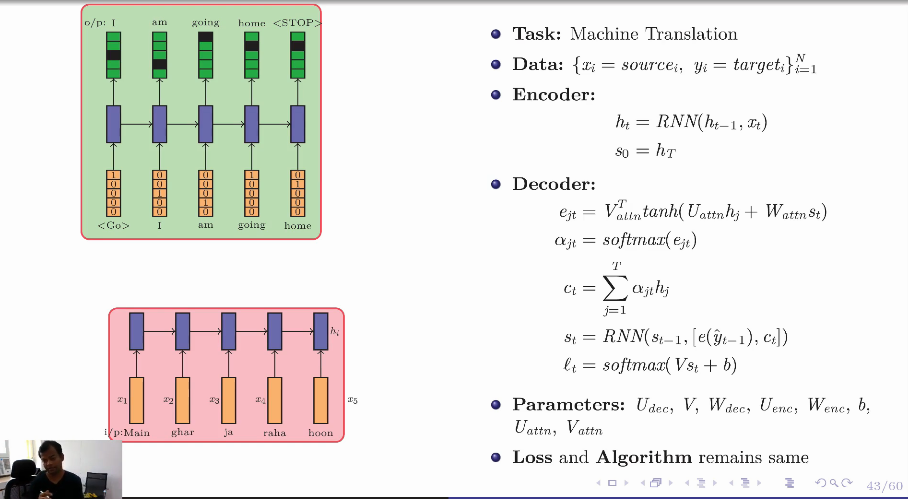
In the Decoder equation their is a correction for $e_{jt}$. Instead of $W_{attn}s_t$, it will be $W_{attn}s_{t-1}$

---

More on Attention

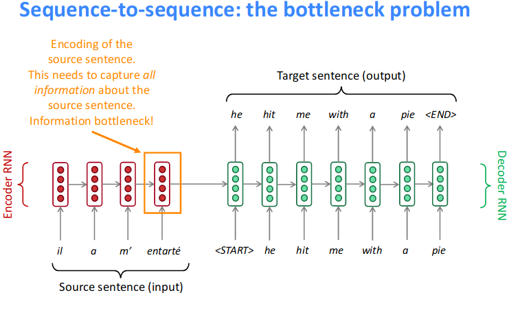
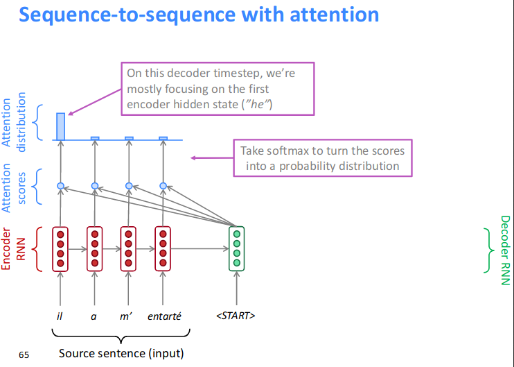
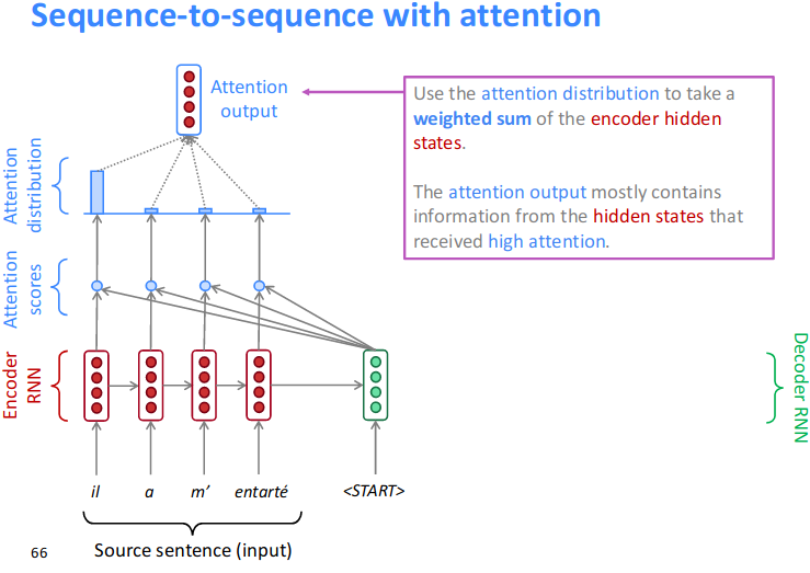
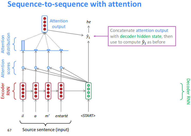
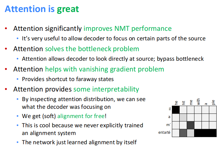
• Attention provides a solution to the bottleneck problem.
• Core idea: on each step of the decoder, use direct connection to the encoderto focus on a particular part of the source sequence

Resource:

• cs224n-2019-lecture08-nmt

---

What is Transformer and it’s pros and cons?

From the Author:

In paper “Attention Is All You Need”, we introduce the Transformer, a novel neural network architecture based on a self-attention mechanism that we believe to be particularly well suited for language understanding.

Natural Language Understanding (NLU): language modeling, machine translation and question answering

• Transformer outperforms both recurrent and convolutional models on academic English to German and English to French translation benchmarks.
• On top of higher translation quality, the Transformer requires less computation to train and is a much better fit for modern machine learning hardware, speeding up training by up to an order of magnitude.

The paper ‘Attention Is All You Need’ describes transformers and what is called a sequence-to-sequence architecture. Sequence-to-Sequence (or Seq2Seq) is a neural net that transforms a given sequence of elements, such as the sequence of words in a sentence, into another sequence.

• One interesting point is, even if it’s used for seq2seq generation, but there is no recurrence part inside the model like the vanilla rnn or lstm.
• So one slight but important part of the model is the positional encoding of the different words. Since we have no recurrent networks that can remember how sequences are fed into a model, we need to somehow give every word/part in our sequence a relative position since a sequence depends on the order of its elements. These positions are added to the embedded representation (n-dimensional vector) of each word.

Pros:

• Faster learning. More GPU efficient unlike the vanilla rnn

The animation below illustrates how we apply the Transformer to machine translation. Neural networks for machine translation typically contain an encoder reading the input sentence and generating a representation of it. A decoder then generates the output sentence word by word while consulting the representation generated by the encoder.

References:

• Paper: Attention is all you need
• Google AI Blog
• Important Blog
• Important: The Illustrated Transformer by Jay Alammar

---

Attention is All You Need

Positional Encoding

Transformer Machine Translation

Transformer Language Pre-training

Multi-head attention

Read the excellent slides from the below reference

Reference:

• CS.Toronto.Lecture16
• Excellent Slide by Alex Smola
• Good summery (even UMLFit)
• Imp slides on Transformer

---

Machine Translation, seq2seq model

Encoder-Decoder Model

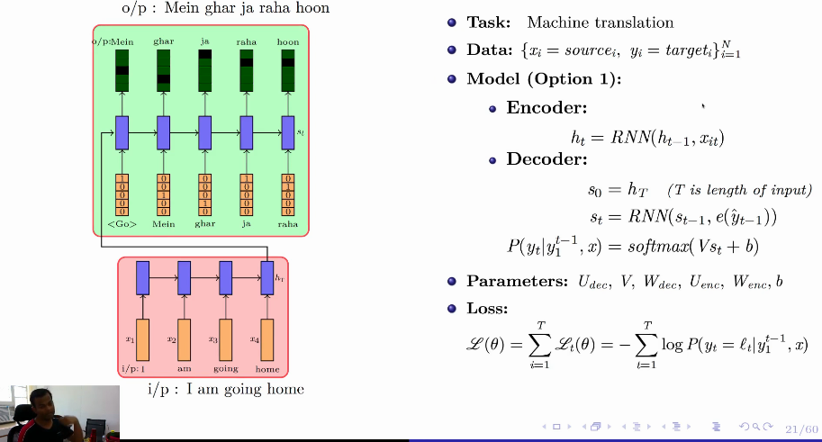
Approach 1:

$h_T$ passed to the $s_0$ of the decoder only.

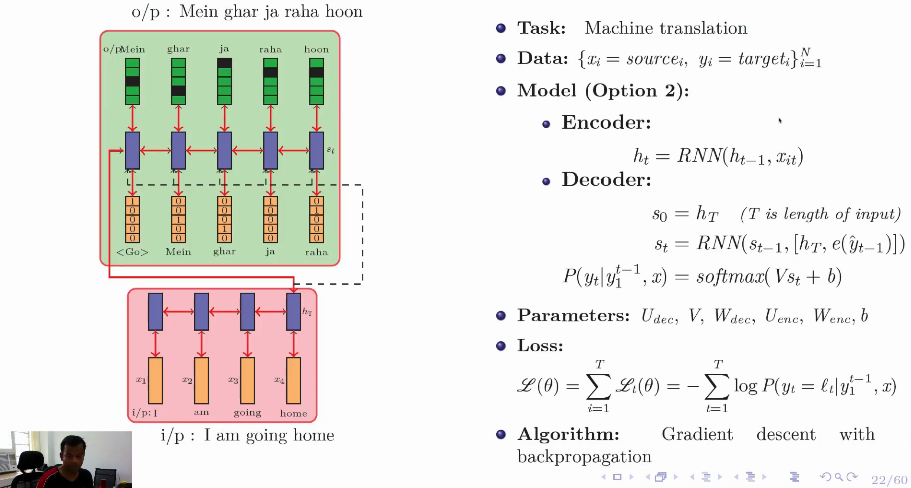
Approach 2:

$h_T$ passed to the every state $s_i$ of decoder.

• Padhai, DL course, Prof. Mikesh, IIT M, Lecture: Encoder Decoder

Neural Machine Translation (NMT)

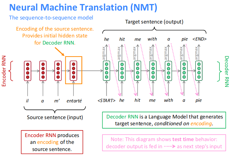
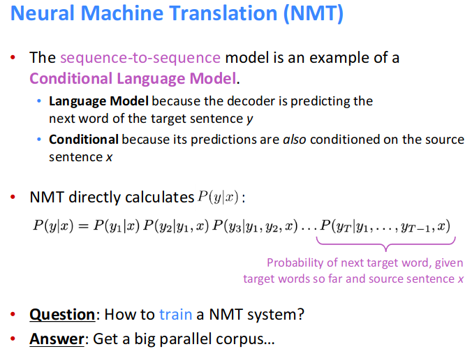
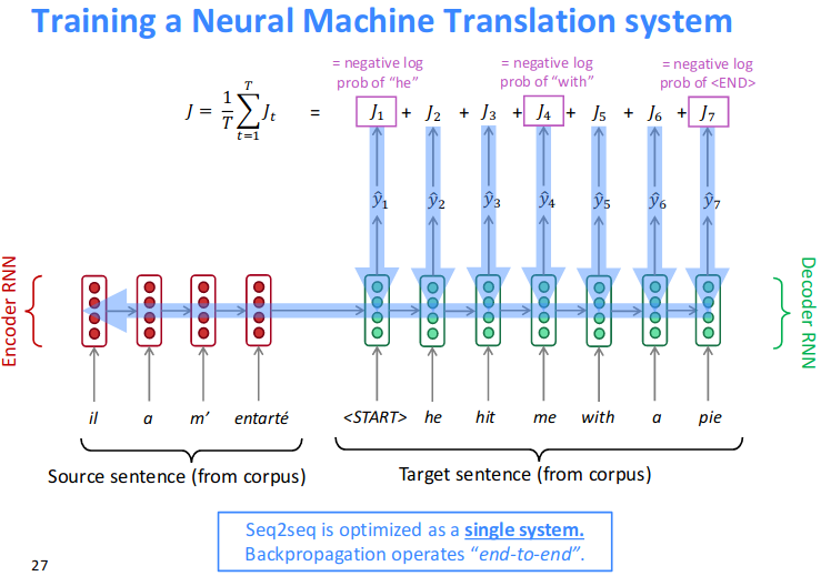
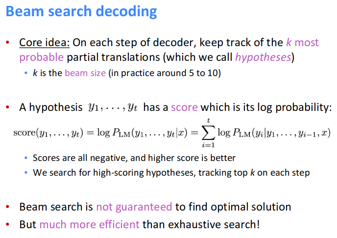
• Neural Machine Translation (NMT)is a way to do Machine Translation with a single neural network.
• The neural network architecture is called sequence-to-sequence(aka seq2seq) and it involves two RNNs.

Resource:

• cs224n-2019-lecture08-nmt

---