Survey - Natural Language Understanding (NLU - Part 1)
Content
- Content
- What is Syntactic and Semantic analysis?
- What is Natural Language Underrstanding?
- Motivation: Why Learn Word Embeddings?
- How to design a basic vector space model?
- What is PMI: Point-wise Mutual Information?
- LSA: Latent Semantic Analysis
- GloVe: Global Vectors
- Word2Vec
- Scaling up with Noise-Contrastive Training
- Retrofitting
- Sentiment Analysis
- What is Lexicon
- Sentiment Dataset
- Art of Tokenization
- Danger of Stemming
- POS tagging
- Stanford Sentiment Treebank (SST)
- Sentiment classifier comparison
- Assessing individual feature selection
- Exercise:
Quick Refresher on Natural Language Understanding
What is Syntactic and Semantic analysis?
Syntactic analysis (syntax) and semantic analysis (semantic) are the two primary techniques that lead to the understanding of natural language. Language is a set of valid sentences, but what makes a sentence valid? Syntax and semantics.
- Syntax is the grammatical structure of the text
- Semantics is the meaning being conveyed.
A sentence that is syntactically correct, however, is not always semantically correct.
- Example, “cows flow supremely” is grammatically valid (subject — verb — adverb) but it doesn’t make any sense.
SYNTACTIC ANALYSIS
Syntactic analysis, also referred to as syntax analysis or parsing.
It is the process of analyzing natural language with the rules of a formal grammar.
Grammatical rules are applied to categories and groups of words, not individual words. Syntactic analysis basically assigns a semantic structure to text.
For example, a sentence includes a subject and a predicate where the subject is a noun phrase and the predicate is a verb phrase. Take a look at the following sentence: “The dog (noun phrase) went away (verb phrase).” Note how we can combine every noun phrase with a verb phrase. Again, it’s important to reiterate that a sentence can be syntactically correct but not make sense.
SEMANTIC ANALYSIS
The way we understand what someone has said is an unconscious process relying on our intuition and knowledge about language itself. In other words, the way we understand language is heavily based on meaning and context. Computers need a different approach, however. The word semantic is a linguistic term and means related to meaning or logic.
![]() Reference:
Reference:
What is Natural Language Underrstanding?
It can be easily understood by the syllabus topic of the course CS224U by Standford. Though over the years the definition has been changed.
2012
- WordNet
- Word sense disambiguation
- Vector-space models
- Dependency parsing for NLU
- Relation extraction
- Semantic role labeling
- Semantic parsing
- Textual inference
- Sentiment analysis
- Semantic composition withvectors
- Text segmentation
- Dialogue
2020
- Vector-space models
- Sentiment analysis
- Relation extraction
- Natural LanguageInference
- Grounding
- Contextual wordrepresentations
- Adversarial testing
- Methods and metrics
![]() Reference:
Reference:
Motivation: Why Learn Word Embeddings?
Image and audio processing systems work with rich, high-dimensional datasets encoded as vectors of the individual raw pixel-intensities for image data, or e.g. power spectral density coefficients for audio data. For tasks like object or speech recognition we know that all the information required to successfully perform the task is encoded in the data (because humans can perform these tasks from the raw data). However, natural language processing systems traditionally treat words as discrete atomic symbols, and therefore cat may be represented as Id537 and dog as Id143. These encodings are arbitrary, and provide no useful information to the system regarding the relationships that may exist between the individual symbols. This means that the model can leverage very little of what it has learned about ‘cats’ when it is processing data about ‘dogs’ (such that they are both animals, four-legged, pets, etc.). Representing words as unique, discrete ids furthermore leads to data sparsity, and usually means that we may need more data in order to successfully train statistical models. Using vector representations can overcome some of these obstacles.
Vector space models (VSMs) represent (embed) words in a continuous vector space where semantically similar (meaningfully similar) words are mapped to nearby points (are embedded nearby each other). VSMs have a long, rich history in NLP, but all methods depend in some way or another on the Distributional Hypothesis,
which states that words that appear in the same contexts share semantic meaning.
The different approaches that leverage this principle can be divided into two categories:
- Count-based methods (e.g. Latent Semantic Analysis),
-
Predictive methods (e.g. neural probabilistic language models like
word2vec).
This distinction is elaborated in much more detail by Baroni et al. 2014 in his great paper Don’t count, predict!, where he compares the context-counting vs context-prediction. In a nutshell:
- Count-based methods first compute the statistics of how often some word co-occurs with its neighbor words in a large text corpus, and then map these count-statistics down to a small, dense vector for each word.
-
Predictive models
directly try to predicta word from its neighbors in terms of learned small, dense embedding vectors (considered parameters of the model).
Word2vec is a particularly computationally-efficient predictive model for learning word embeddings from raw text. It comes in two flavors, the Continuous Bag-of-Words model (CBOW) and the Skip-Gram model.
- Algorithmically, these models are similar, except that CBOW predicts target words (e.g. ‘mat’) from source context words (‘the cat sits on the’), while the skip-gram does the inverse and predicts source context-words from the target words.
This inversion might seem like an arbitrary choice, but statistically it has different effect.
- CBOW smoothes over a lot of the distributional information (by treating an entire context as one observation). For the most part, this turns out to be a useful thing for smaller datasets.
- Skip-gram treats each context-target pair as a new observation, and this tends to do better when we have larger datasets.
![]() Reference:
Reference:
How to design a basic vector space model?
What is PMI: Point-wise Mutual Information?
The idea behind the NLP algorithm is that of transposing words into a vector space, where each word is a D-dimensional vector of features. By doing so, we can compute some quantitative metrics of words and between words, namely their cosine similarity.
Problem: How to understand whether two (or more) words actually form a unique concept?
Example: Namely, consider the expression ‘social media’: both the words can have independent meaning, however, when they are together, they express a precise, unique concept.
Nevertheless, it is not an easy task, since if both words are frequent by themselves, their co-occurrence might be just a chance. Namely, consider the name ‘Las Vegas’: it is not that frequent to read only ‘Las’ or ‘Vegas’ (in English corpora of course). The only way we see them is in the bigram Las Vegas, hence it is likely for them to form a unique concept. On the other hand, if we think of ‘New York’, it is easy to see that the word ‘New’ will probably occur very frequently in different contexts. How can we assess that the co-occurrence with York is meaningful and not as vague as ‘new dog, new cat…’?
The answer lies in the Pointwise Mutual Information (PMI) criterion. The idea of PMI is that we want to
quantify the likelihood of co-occurrence of two words, taking into account the fact that it might be caused by the frequency of the single words.
Hence, the algorithm computes the ($\log$) probability of co-occurrence scaled by the product of the single probability of occurrence as follows:
where $w_a$ and $w_b$ are two words.
Now, knowing that, when $w_a$ and $w_b$ are independent, their joint probability is equal to the product of their marginal probabilities, when the ratio equals 1 (hence the log equals 0), it means that the two words together don’t form a unique concept: they co-occur by chance.
On the other hand, if either one of the words (or even both of them) has a low probability of occurrence if singularly considered, but its joint probability together with the other word is high, it means that the two are likely to express a unique concept.
PMI is the re-weighting of the entire count matrix
Let’s focus on the last expression. As you can see, it’s the conditional probability of $w_b$ given $w_a$ times $\frac{1}{p(w_b)}$. If $w_b$ and $w_a$ are independent, there is no meaning to the multiplication (it’s going to be zero times something). But if the conditional probability is larger than zero, $p(w_b \vert w_a) > 0$, then there is a meaning to the multiplication. How important is the event $W_b = w_b$? if $P(W_b = w_b) = 1$ then the event $W_b = w_b$ is not really important is it? think a die which always rolls the same number; there is no point to consider it. But, If the event $W_b = w_b$ is fairly rare → $p(w_b)$ is relatively low → $\frac{1}{p(w_b)}$ is relatively high → the value of $p(w_b \vert w_a)$ becomes much more important in terms of information. So that is the first observation regarding the PMI formula.
![]() Reference:
Reference:
LSA: Latent Semantic Analysis
Note: LSA and [LS (Latent Semantic Indexing) are mostly used synonymously, with the information retrieval community usually referring to it as LSI. LSA/LSI uses SVD to decompose the term-document matrix $A$ into a term-concept matrix $U$, a singular value matrix $S$, and a concept-document matrix $V$ in the form: $A = USV’$
- One of the oldest and most widely used dimensionality reduction method.
- Also known as truncated SVD
- Standard baseline, often very tough to beat.
Related dimensionality reduction technique
- PCA
- NNMF
- Probabilistic LSA
- LDA
- t-SNE
For more details check this blog from msank
![]() Reference:
Reference:
GloVe: Global Vectors
Read this amazing paper by Pennington et al. (2014) [1]
GloVe [1] is an unsupervised learning algorithm for obtaining vector representations for words. Training is performed on aggregated global word-word co-occurrence statistics from a corpus, and the resulting representations showcase interesting linear substructures of the word vector space.
The authors of Glove show that the ratio of the co-occurrence probabilities of two words (rather than their co-occurrence probabilities themselves) is what contains information and aim to encode this information as vector differences.
To achieve this, they propose a weighted least squares objective $J$ that directly aims to minimize the difference between the dot product of the vectors of two words and the logarithm of their number of co-occurrences:
where $w_i$ and $b_i$ are the word vector and bias respectively of word $i$, $\tilde{w_j}$ and $b_j$ are the context word vector and bias respectively of word $j$, $X_{ij}$ is the number of times word $i$ occurs in the context of word $j$, and $f$ is a weighting function that assigns relatively lower weight to rare and frequent co-occurrences.
Main Idea:
The objective is to learn vectors for words such that their dot product is proportional to their probability of co-occurrence.
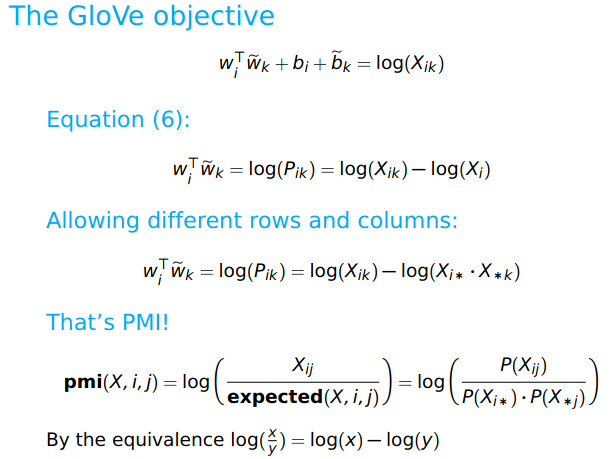
- $w_i$: row embedding
- $w_k$: column embedding
- $X_{ik}$: Co-occurrence count
- $\log(P_{ik})$: log of co-occurrence probability
- $\log(X_{ik})$: log of co-occurrence count
- $\log(X_i)$: log of row probability
Their dot products are the 2 primary terms + 2 bias terms.
And the idea is that should be equal to (at-least proportional to) the log of the co-occurrence probability.
Equation 6 tells that the dot product is equal to the difference of of two log terms and if re-arrange them they looks very similar to PMI !! Where PMI is the re-weighting of the entire count matrix.
The Weighted GloVe objective
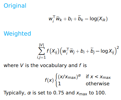
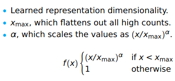
Weighted by the function $f()$. Which is flattening out and rescaleing the co-occurrence count $X_{ik}$ values.
Say the co-occurrence count vector is like this v = [100 99 75 10 1]. Then $f(v)$ is [1.00 0.99 0.81 0.18 0.03].
What’s happening behind the scene (BTS)?
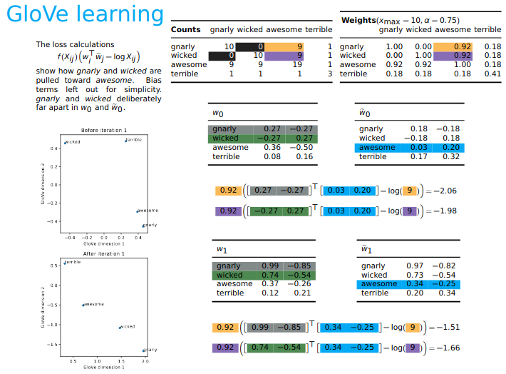
Example:
Word wicked and gnarly (positive slang) never co-occur. If you look at the left plot in the above image, then you see, what GLoVe does is, it pushes both wicked and gnarly away from negative word terrible and moves them towards positive word awsome. Because even if wicked and gnarly don’t occur together, they have co-occurrence with positive word awsome. GloVe thus achieves this latent connection.
Note: Glove transforms the raw count distribution into a normal distribution which is essential when you train deep-learning model using word-embedding as your initial layer. It’s essential because the embedding values have constant mean and variance and this is a crucial part for training any deep-learning model. The weight values while passing through different layers should maintain their distribution. That’s why GloVe does so well as an input to another system.
![]() Reference:
Reference:
-
CS224U Slide

-
CS224U Youtube

-
[1] Paper: Glove: Global Vectors for Word Representation, EMNLP 2014

- On word embeddings - Part 1: Sebastian Ruder
- Language Model: CS124
Word2Vec
- Introduced by Mikolov et al. 2013 [2]
- Goldberg and Levy 2014 [3] identified the relation between
word2vecandPMI - Gensim package has a highly scalable implementation
We are going to summarize $2$ papers
-
Efficient Estimation of Word Representations in Vector Space [1]
- Author: Tomas Mikolov, Kai Chen, Greg Corrado, Jeffrey Dean
- Paper
-
Distributed Representations of Words and Phrases and their Compositionality [2]
- Author: Tomas Mikolov, Ilya Sutskever, Kai Chen, Greg Corrado, Jeffrey Dean
- Paper
-
Distributed representations of wordsin avector spacehelp learning algorithms to achieve better performance in natural language processing tasks bygrouping similar words. - Earlier there were label encoding, binarization or one-hot-encoding. Those were
sparse vector representation. But the Skip-gram model helps to represent the words ascontinuous dense vector. - The problem with label encoding, one-hot-encoding type vector representation is that, they don’t capture the correlation (very loosely speaking) with each other. The correlation groups the words in terms of their hidden or latent meaning.
Example
Let’s say we have 4 words: dog, cat, chair and table.
If we apply one-hot-encoding then:
- dog: [0, 0]
- cat: [0, 1]
- chair: [1, 0]
- table: [1, 1]
The above is a random order. We can put in any random order that will not be a problem. Because all 4 words are not related in the vector space.
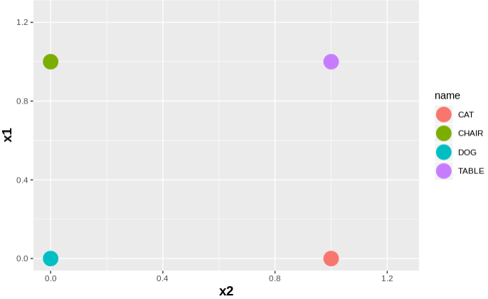
However cat and dog are from type animal and chair and table are from type furniture. So it would have been very good if in the vector space they were grouped together and their vectors are adjusted accordingly.
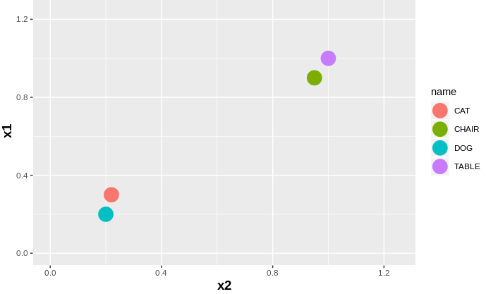
Now there are many methods to learn these kind of representation. But at present 2 popular ones are CBOW: Continuous Bag of Words and Skip-gram model.
Both are kind of complement of each other.
Say, we have a sentence $S = w_1 w_2 w_3 w_4 w_5$ where $w_i$ are words. Now say we pick word $w_3$ as our candidate word for which we are trying to get the dense vector. Then the remaining words are neighbor words. These neighbor words denote the context for the candidate words and the dense vector representation capture these properties.
- Sentence $S = w_1 w_2 w_3 w_4 w_5$
- Candidate: $w_3$
- Neighbor: $w_1 w_2 w_4 w_5$
Objective
The train objective is to learn word vector representation that are good at predicting the nearby words.
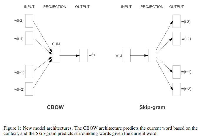
CBOW Objective: Predicts the candidate word $w_3$ based on neighbor words $w_1 w_2 w_4 w_5$.
Skip-gram Objective: Predicts the Neighbor words $w_1 w_2 w_4 w_5$ based on candidate word $w_3$
Word2Vec
Let us now introduce arguably the most popular word embedding model, the model that launched a thousand word embedding papers: word2vec, the subject of two papers by Mikolov et al. in 2013.
As word embeddings are a key building block of deep learning models for NLP, word2vec is often assumed to belong to the same group. Technically however, word2vec is not be considered to be part of deep learning, as its architecture is neither deep nor uses non-linearities (in contrast to Bengio’s model and the C&W model).
In their first paper [4], Mikolov et al. propose two architectures for learning word embeddings that are computationally less expensive than previous models.
In their second paper [2], they improve upon these models by employing additional strategies to enhance training speed and accuracy.
These architectures offer two main benefits over the C&W model [6] and Bengio’s language model [5]:
- They do away with the expensive hidden layer.
- They enable the language model to take additional context into account.
As we will later show, the success of their model is not only due to these changes, but especially due to certain training strategies.
Side-note: word2vec and GloVe might be said to be to NLP what VGGNet is to vision, i.e. a common weight initialization that provides generally helpful features without the need for lengthy training.
In the following, we will look at both of these architectures:
Continuous bag-of-words (CBOW)
Mikolov et al. thus use both the $n$ words before and after the target word $w_t$ to predict it. They call this continuous bag-of-words (CBOW), as it uses continuous representations whose order is of no importance.
The objective function of CBOW in turn is only slightly different than the language model one:
where $w_{t-n}^{t-1}=w_{t-n} , \cdots , w_{t-1}$ and $w_{t+1}^{t+n}=w_{t+1}, \cdots , w_{t+n}$
The Skip-gram model
While CBOW can be seen as a precognitive language model, skip-gram turns the language model objective on its head: Instead of using the surrounding words to predict the centre word as with CBOW, skip-gram uses the centre word to predict the surrounding words
The training objective of the Skip-gram model is to find word representations that are useful for predicting the surrounding words in a sentence or a document. More formally, given a sequence of training words $w_1, w_2, w_3, \dots , w_T$, the objective of the Skip-gram model is to maximize the average log probability, i.e
where $c$ is the size of the training context (which can be a function of the center word $w_t$). Larger $c$ results in more training examples and thus can lead to a higher accuracy, at the expense of the training time.
The basic Skip-gram formulation defines $p(w_{t+j} \vert w_t)$ using the softmax function.
- A computationally
efficient approximationof the full softmax is the hierarchical softmax. The main advantage is that instead of evaluating $W$ output nodes in the neural network to obtain the probability distribution, it is needed to evaluate only about $\log_2(W)$ nodes. - The hierarchical softmax uses a binary tree representation of the output layer with the W words as its leaves and, for each node, explicitly represents the relative probabilities of its child nodes. These define a random walk that assigns probabilities to words.
- Such representation makes the learning faster using distributed technique.
Word2vec: from corpus to labeled data
- input sentence:
it was the best of times it was the worst of times... - window size = 2
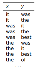
Earlier in LSA and others, it was count-based co-occurrence, but here it’s like positional co-occurrence, thus bypassing the task of creating the count-matrix.
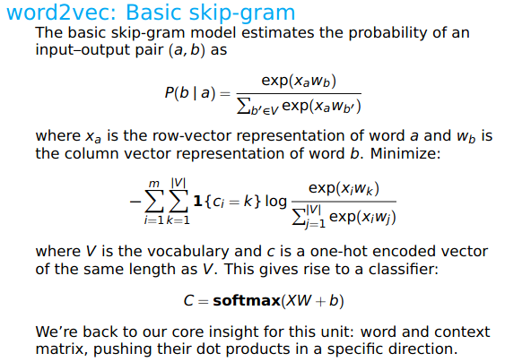
- $C$ is a label vector for individual example and it’s one-hot-encoded. But it has the dimensionality of the entire Vocabulary $V$. Where size of $V$ is very big and therefore, it’s difficult to train. But that’s the intuition, that after creating a labelled dataset apply standard machine learning classifier to predict those labels. However, this is the backbone of the word2vec variant SkipGram model.
The objective of the model is to push the
dot productin a particular direction i.e towards words which co-occur a lot.
To bypass the training issue a variant of SkipGram is used.
Word2vec: noise contrastive estimation

Sum of 2 separate objective, each one of them is binary. The left side is for those words which actually co-occur. And then we sample some negative instances (meaning the word pair that doesn’t co-occur) which are used in the right side objective.
![]() Reference:
Reference:
- [2] Paper: Distributed Representations of Words and Phrases and their Compositionality
- [3] Paper: Neural Word Embeddingas Implicit Matrix Factorization
- [4] Mikolov, T., Corrado, G., Chen, K., & Dean, J. (2013). Efficient Estimation of Word Representations in Vector Space. (ICLR 2013)
- [5] Bengio, Y., Ducharme, R., Vincent, P., & Janvin, C. (2003). A Neural Probabilistic Language Model. The Journal of Machine Learning Research
- [6] Collobert, R., & Weston, J. (2008). A unified architecture for natural language processing. ICML ’08,
- [7] Pennington, J., Socher, R., & Manning, C. D. (2014). Glove: Global Vectors for Word Representation, EMNLP 2014
- CS224u Youtube Lecture
Scaling up with Noise-Contrastive Training
Neural probabilistic language models are traditionally trained using the maximum likelihood (ML) principle to maximize the probability of the next word $w_t$ (for target) given the previous words $h$ (for history) in terms of a softmax function,
where $\text{score}(w_t, h)$ computes the compatibility of word $w_t$ with the context $h$ (a dot product is commonly used). We train this model by maximizing its log-likelihood on the training set, i.e. by maximizing
- $w’$ is a word
- $V$ is the vocabulary set
This yields a properly normalized probabilistic model for language modeling. However this is very expensive, because we need to compute and normalize each probability using the score for all other $V$ words $w’$ in the current context $h$, at every training step.
On the other hand, for feature learning in word2vec we do not need a full probabilistic model. The CBOW and skip-gram models are instead trained using a binary classification objective (logistic regression) to discriminate the real target words $w_t$ from $k$ imaginary (noise) words $\tilde w$, in the same context. We illustrate this below for a CBOW model. For skip-gram the direction is simply inverted.
Mathematically, the objective (for each example) is to maximize
- where $Q_\theta(D=1 \vert w, h)$ is the binary logistic regression probability under the model of seeing the word $w$ in the context $h$ in the dataset $D$, calculated in terms of the learned embedding vectors $\theta$.
- In practice the author approximates the expectation by drawing $k$ contrastive words (contrasting/different words) from the noise distribution (i.e. we compute a Monte Carlo average).
This objective is maximized when the model assigns high probabilities to the real words, and low probabilities to noise words. Technically, this is called Negative Sampling [8], and there is good mathematical motivation for using this loss function:
- The updates it proposes approximate the updates of the softmax function in the limit.
- But computationally it is especially appealing because computing the loss function now scales only with the number of noise words that we select ($k$), and not all words in the vocabulary ($V$).
- This makes it much faster to train. The author uses the very similar
noise-contrastive estimation[9] (NCE) loss.
![]() Reference:
Reference:
-
TensorFlow: Vector Representations of Words


- [8] Paper: Distributed Representations of Words and Phrases and their Compositionality
- [9] Paper: Learning word embeddings efficiently with noise-contrastive estimation
Retrofitting
Central goals:
- Distributional representations are powerful and easy, but they tend to reflect only similarity (synonymy, connotation).
- Structured resources are sparse and hard to obtain, but they support learning rich, diverse,
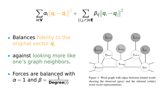
semanticdistinctions. - Can we have the best of both world? Answer is YES using Retrofitting.
- Read the original paper from Faruqui et al 2015, NAACL best paper


![]() Reference:
Reference:
Sentiment Analysis
Core Reading
- Sentiment Treebank - Richard Socher, EMNLP 2013
- Opinion mining and sentiment analysis - Pang and Lee (2008)
- A Primer on Neural Network Models for Natural Language Processing - Goldberg 2015
Introduction
Sentiment analysis seems simple at first but turns out to exhibit all of the complexity of full natural language understanding. To see this, consider how your intuitions about the sentiment of the following sentences can change depending on perspective, social relationships, tone of voice, and other aspects of the context of utterance:
- There was an earthquake in LA.
- The team failed the physical challenge. (We win/lose!)
- They said it would be great. They were right/wrong.
- Many consider the masterpiece bewildering, boring, slow-moving or annoying.
- The party fat-cats are sipping their expensive, imported wines.
- Oh, you’re terrible!
Related paper
-
 Subjectivity - Pang and Lee 2008
-
 Bias - Recasens et al. 2013
-
 Stance - Anand et al. 2011
-
 Abusive Language Detection - Nobata et al. 2016
-
 Sarcasm - Khodak et al. 2017
-
 Deception and Betrayal - Niculae et al. 2015
-
 Online Troll - Cheng et al. CSCW 2017
-
 Polarization - Gentzkow et al. 2019
-
 Politeness - Danescu-Niculescu-Mizil et al. 2013
-
 Linguistic alignment - Doyle et al. 2013
*Dataset available for these paper
![]() Reference:
Reference:
What is Lexicon
A word to meaning dictionary
Sentiment Dataset
Art of Tokenization
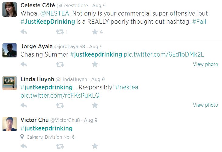
Normal words are fine for tokenization. But it becomes problematic when you process social media post, e.g Tweet.
-
whitespacetokenization is Okay. Basic. Preserve emoticons. -
treebanktokenizer - most systems are using.- Destroys hashtags, http link emoticons
-
sentiment awaretokenizationnltk.tokenize.casual.TweetTokenizer- Isolate emoticon, respect domain specific tweet markup, capture multi-word expression, preserves capitalization where seems meaningful.
Different tokenization has impact on the final nlp task.
![]() Reference:
Reference:
Danger of Stemming
- Stemming is heuristically collapsing words together by trimming of their ends. The idea is, this is helping you to collapse
morphologicalvariance. -
porterandlancasterdestroy too many sentiment distinctions. -
wordnetis better but still not best. - All comparative and superlative adjectives are stripped down to their base form
-
Sentiment-awaretokenizer beats bothporterandlancaster
Question
Does stemming work on misspelling words?
Ans: Stemming is a set of rules and they are not intelligent. So whatever input you feed to them, if the rules are applicable, then they will be applied. However, for modern NLU model, misspelling words are not that much of a problem due to dense representations of words generated from the context. Therefore, if you have a common misspelling, then their word representation will be similar to the actual correct word. And this is one of the selling point of the modern NLU papers which state that no need of spell checker as preprocessing steps as the system will gracefully recover from that due to context aware word vector representation.
POS tagging
POS tagging helps in improving sentiment classification task. Because there are words for which if multiple pos tags are available, then sentiment of different tags are different.
Example:
-
fine: if Adjective POSITIVE, if Noun then NEGATIVE
But even that Sentiment distinctions transcends (goes beyond) parts of speech.
Stanford Sentiment Treebank (SST)
Most sentiment prediction systems work just by looking at words in isolation, giving positive points for positive words and negative points for negative words and then summing up these points. Problem: the order of words is ignored and important information is lost.
In constrast, our new deep learning model actually
builds up a representation of whole sentences based on the
sentence structure.
It computes the sentiment based on how words compose the meaning of longer phrases.

This way, the model is not as easily fooled as previous models. For example, our model learned that funny and witty are positive but the following sentence is still negative overall:
This movie was actually neither that funny, nor super witty.
The underlying technology of this demo is based on a new type of Recursive Neural Network that builds on top of grammatical structures.
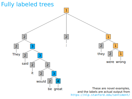
Sentiment from bottom up is projected towards the top.
-
 positive
 -
 neutral
 -
 negative
SST-5 consists of $11855$ sentences extracted from movie reviews with fine-grained sentiment labels $[1–5]$, as well as $215154$ phrases that compose each sentence in the dataset.
The raw data with phrase-based fine-grained sentiment labels is in the form of a tree structure, designed to help train a Recursive Neural Tensor Network (RNTN) from their 2013 paper. The component phrases were constructed by parsing each sentence using the Stanford parser (section 3 in the paper) and creating a recursive tree structure as shown in the below image. A deep neural network was then trained on the tree structure of each sentence to classify the sentiment of each phrase to obtain a cumulative sentiment of the entire sentence.
![]() Reference:
Reference:
- Stanford sentiment
- Blog
- Check the noebooks on sst from the course website
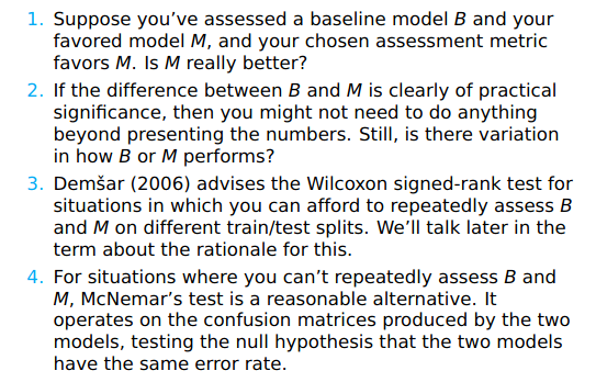
Sentiment classifier comparison
![]() Reference:
Reference:
Assessing individual feature selection
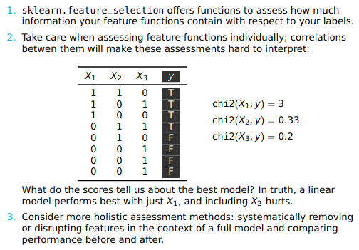
These kind of feature selection in the presence of correlated features are hard to interpret. So handle with care.
Exercise:
- What is UMLFit ?
- What is U-Net