Content

1. Content
2. When we should accept an Algorithm and when we shouldn’t?
   1. K-Means:
   2. Hierarchical Clustering
3. Bayesian Analysis
4. How to interpret $R^2$ ?
5. Linear and Bayesian modeling in R: Predicting movie popularity
6. Bayesian Linear Regression
7. What is Sampling methods?
   1. Sampling from a probability distribution
8. What is Variational Inference?
9. What is Graphical Model (GM)?
10. What is Markov Model?
    1. Application: Language modeling
11. Hidden Markov Model
    1. Application of HMMs
12. Undirected graphical models (Markov random fields)
13. Conditional Random Field
14. Confidence Inteval and Normal Approximation
15. Exercise:

---

When we should accept an Algorithm and when we shouldn’t?

Each algorithm is based on some assumption which is applicable to some scenario. Now if the assumption fails in some scenario, then the Algorithm will fail there.

Example:

K-Means:

Assumptions:

• k-means assume the variance of the distribution of each attribute (variable) is spherical;

• All variables have the same variance;
• The prior probability for all $k$ clusters are the same, i.e. each cluster has roughly equal number of observations;

Drawbacks:

• If any one of these 3 assumptions is violated, then k-means will fail.
• Number of cluster needs to know beforehand.
• The clusters should be non-overlapping.

Reference:

• kmeans-free-lunch

Hierarchical Clustering

Hierarchical clustering is the hierarchical decomposition of the data based on group similarities

Assumptions:

1. There should be hierarchical relationship in the data, i.e a smaller cluster is nested within a bigger cluster.

The term hierarchical refers to the fact that clusters obtained by cutting the dendrogram at a given height are necessarily nested within the clusters obtained by cutting the dendrogram at any greater height.

Pros:

• No need to know the number of cluster beforehand.

Cons:

• If the data doesn’t satisfy Assumption 1, then it’s not recommended to use Hierarchical Clustering. For example: In an arbitary dataset 120 people, 60 male and 60 female and they are from US, ITALY and INDIA with (40 people/Nationality). Here gender and nationality are not related so there is no nesting relation here and therefore, it’s unwise to use Hierarchical Clustering here.

• Both K-Means and Hierarchical Clustering techniques are hard cluster. They force each datapoint to belong to any cluster even if it’s an outlier. So the final clustering may be distorted. So these models are sensitive to outlier.
• In such scenario, soft cluster like Mixture Models are more appropriate.

Reference:

• Book: ISL Chapter 10, Page 394

---

Bayesian Analysis

$P(Hyp \vert Data) = \frac{P(Data \vert Hyp) P(Hyp)}{P(Data)}$ $posterior \propto Likelihood \times prior$

• $p(Hyp)$ is the probability of the hypothesis before we see the data, called the prior probability, or just prior.
• $p(Hyp\vert Data)$ is our goal, this is the probability of the hypothesis after we see the data, called the posterior.
• $p(Data \vert Hyp)$ is the probability of the data under the hypothesis, called the likelihood.

There is an element which is key when we want to build a model under Bayesian approach: the Bayes factor . The Bayes factor is the ratio of the likelihood probability of two competing hypotheses (usually null and alternative hypothesis) and it helps us to quantify the support of a model over another one.

• however, the prior starts to lose weight when we add more data

---

How to interpret $R^2$ ?

Specifically, this linear regression is used to determine how well a line fits’ to a data set of observations, especially when comparing models. Also, it is the fraction of the total variation in y that is captured by a model.

..it captures how much variability of target variable, the model is capturing…

$SS_{tot} = \Sigma_i (y_i - \bar y)^2$ $SS_{res} = \Sigma_i (y_i - \hat{y_i})^2$

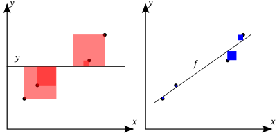
where $\hat{y_i} = f(x_i)$

• If the adjusted $R^2$ of our final model is only $0.3595$, so this means that $35.95$% of the variability is explained by the model.

Reference:

• Wiki

---

Linear and Bayesian modeling in R: Predicting movie popularity

Reference

• TDS Blog

---

Bayesian Linear Regression

Bayesian linear regression allows a fairly natural mechanism to survive insufficient data, or poor distributed data. It allows you to put a prior on the coefficients and on the noise so that in the absence of data, the priors can take over. More importantly, you can ask Bayesian linear regression which parts (if any) of its fit to the data is it confident about, and which parts are very uncertain (perhaps based entirely on the priors).

Read this book’s chapter 6 thoroughly link .

Reference:

• Bayesian
• Chapter 6: introduction-to-bayesian-regression

---

What is Sampling methods?

These are approximation methods to solve complex probabilistic model, which are difficult to solve in polinomial time with simpler methods.

There exist two main families of approximate algorithms:

• Variational methods: Formulate inference as an optimization problem
• Sampling methods: Which produce answers by repeatedly generating random numbers from a distribution of interest.

Sampling from a probability distribution

Q: How we might sample from a multinomial distribution with $k$ possible outcomes and associated probabilities $\theta_1, \dots , \theta_k$.

Reduce sampling from a multinomial variable to sampling a single uniform variable by subdividing a unit interval into $k$ regions with region $i$ having size $\theta_i$. We then sample uniformly from $[0,1]$ and return the value of the region in which our sample falls.

Reducing sampling from a multinomial distribution to sampling a uniform distribution in [0,1].

• Sampling from a distribution lets us perform many useful tasks, including marginal and MAP inference, as well as computing integrals of the form

$E_{x \sim p}[f(x)] = \sum_x f(x) p(x)$

Algorithms that construct solutions based on a large number of samples from a given distribution are referred to as Monte Carlo (MC) methods.

For different type of sampling technique check here.

Reference

• Sampling Methods CS228

---

What is Variational Inference?

• Variational inference methods take their name from the calculus of variations, which deals with optimizing functions that take other functions as arguments.

Inference in probabilistic models is often intractable, and we learned about algorithms that provide approximate solutions to the inference problem (e.g. marginal inference) by using subroutines that involve sampling random variables.

Unfortunately, these sampling-based methods have several important shortcomings.

So an alternative approach to approximate inference is by using the variational family of algorithms.

The main idea of variational methods is to cast inference as an optimization problem.

Inference as Optimization: Suppose we are given an intractable probability distribution $p$. Variational techniques will try to solve an optimization problem over a class of tractable distributions $Q$ in order to find a $q\in Q$ that is most similar to $p$. We will then query $q$ (rather than $p$) in order to get an approximate solution.

• Variational inference methods often scale better and are more amenable to techniques like stochastic gradient optimization, parallelization over multiple processors, and acceleration using GPUs.

To formulate inference as an optimization problem, we need to choose an approximating family $Q$ and an optimization objective $J(q)$. This objective needs to capture the similarity between $q$ and $p$; the field of information theory provides us with a tool for this called the Kullback-Leibler (KL) divergence.

$ KL(q\|p) = \sum_x q(x) \log \frac{q(x)}{p(x)} = E_{x \sim q}[f(x)] $

where $f(x)$ is $\log \frac{q(x)}{p(x)}$

Reference

• High Level Understanding
• Important CS228

---

What is Graphical Model (GM)?

In graphical models, each vertex represents a random variable, and the graph gives a visual way of understanding the joint distribution of the entire set of random variables.

They can be useful for either unsupervised or supervised learning.

• Directed graphical models or Bayesian networks; these are graphical models in which the edges have directional arrows (but no directed cycles). Directed graphical models represent probability distributions that can be factored into products of conditional distributions, and have the potential for causal interpretations.

*In case the above link is broken, click here

Naive Bayes and Logistic Regression can be thought as Bayes Nets

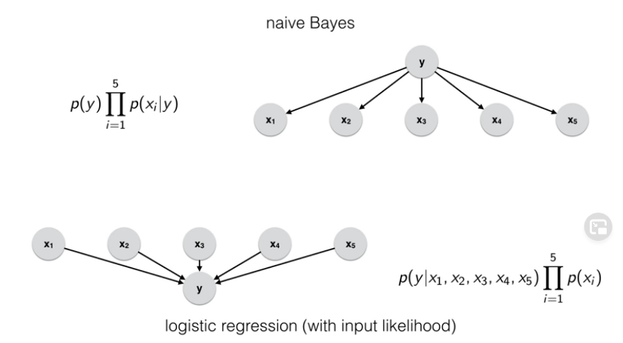
• Undirected graphical models, also known as Markov random fields (MRF) or Markov networks.

*In case the above link is broken, click here

• GMs tend to fall into two broad classes – those useful in modelling, and those useful in representing inference algorithms.
  • For modelling, Belief Networks, Markov Networks, Chain Graphs and Influence Diagrams are some of the most popular.
  • For inference one typically compiles a model into a suitable GM for which an algorithm can be readily applied. Such inference GMs include Factor Graphs, Junction Trees and Region Graphs.

Reference:

• [ch 17, elements of statistical learning]
• [ch 4, Bayesian Reasoning and ML by D. Barber]

---

What is Markov Model?

Markov Networks, for example, are particularly suited to modelling marginal dependence and conditional independence.

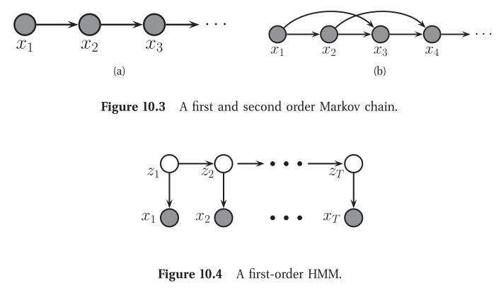
Figure 10.3(a) illustrates a first-order Markov chain as a DAG. Of course, the assumption that the immediate past, $x_{t−1}$, captures everything we need to know about the entire history, $x_{1:t−2}$,is a bit strong. We can relax it a little by adding a dependence from $x_{t−2}$ to $x_t$ as well; this is called a second order Markov chain, and is illustrated in Figure 10.3(b).

The corresponding joint distribution is:

$ P(x_{1:T}) = P(x_1, x_2) \prod_{t=3}^T P(x_t \vert x_{t-1}, x_{t-2}) $

• Unfortunately, even the second-order Markov assumption may be inadequate if there are long-range correlations amongst the observations.
• An alternative approach is to assume that there is an underlying hidden process, that can be modeled by a first-order Markov chain, but that the data is a noisy observation of this process. The result is known as a hidden Markov model or HMM, and is illustrated in Figure 10.4.
• Here $z_t$ is known as a hidden variable at time t, and $x_t$ is the observed variable. (We put “time” in quotation marks, since these models can be applied to any kind of sequence data, such as genomics or language, where t represents location rather than time.) The conditional probability distribution (CPD) $p(z_t \vert z_{t−1})$ is the transition model, and the CPD $p(x_t \vert z_t)$ is the observation model.

---

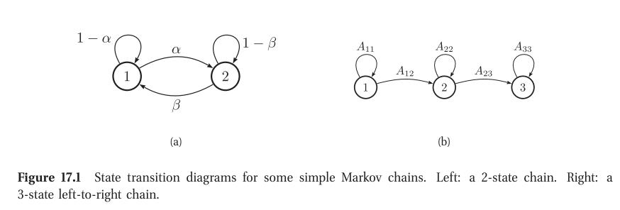
Application: Language modeling

One important application of Markov models is to make statistical language models, which are probability distributions over sequences of words. We define the state space to be all the words in English (or some other language).

• The marginal probabilities $p(X_t = k)$ are called unigram statistics.
• If we use a first-order Markov model, then $p(X_t = k \vert X_{t−1} = j)$ is called a bigram model.

• If we use a second-order Markov model, then $p(X_t = k \vert X_{t−1} = j , X_{t−2} = i)$ is called trigram model.

• Sentence completion: A language model can predict the next word given the previous words in a sentence.
• Data compression: Any density model can be used to define an encoding scheme, by assigning short codewords to more probable strings. The more accurate the predictive model, the fewer the number of bits it requires to store the data.
• Text classification: Any density model can be used as a class-conditional density and hence turned into a (generative) classifier.
  • Note that using a 0-gram class-conditional density (i.e., only unigram statistics) would be equivalent to a naive Bayes classifier.
• Automatic essay writing: One can sample from $p(x_{1:t})$ to generate artificial text (i.e. sample from joint distribution of the text). This is one way of assessing the quality of the model.

Example: 4-gram based language model

SAYS IT’S NOT IN THE CARDS LEGENDARY RECONNAISSANCE BY ROLLIE DEMOCRACIES UNSUSTAINABLE COULD STRIKE REDLINING VISITS TO PROFIT BOOKING WAIT HERE AT MADISON SQUARE GARDEN COUNTY COURTHOUSE WHERE HE HAD BEEN DONE IN THREE ALREADY IN ANY WAY IN WHICH A TEACHER

Example output from an 4-gram word model, trained using backoff smoothing on the Broadcast News corpus. The first 4 words are specified by hand, the model generates the 5th word, and then the results are fed back into the model.

• Later ((Tomas et al. 2011) describes a much better language model, based on recurrent neural networks, which generates much more semantically plausible text.)

Another application: Google’s PageRank algorithm for web page ranking

Read the chapter for MLE of Markov Model.

Reference:

• [murphy, sec. $10.2.2$ and ch: $17$]

---

Hidden Markov Model

A hidden Markov model or HMM consists of a discrete-time, discrete-state Markov chain, with hidden states $z_t \in {1, \dots ,K}$, plus an observation model $p(x_t \vert z_t)$.

The corresponding joint distribution has the form

$ p(z_{1:T}, x_{1:T})= p(z_{1:T})p(x_{1:T} \vert z_{1:T})=[p(z_1) \prod_{t=2}^T p(z_t \vert z_{t-1})][\prod_{t=1}^T p(x_t \vert z_t)] $

Application of HMMs

HMMs can be used as black-box density models on sequences. They have the advantage over Markov models in that they can represent long-range dependencies between observations, mediated via the latent variables. In particular, note that they do not assume the Markov property holds for the observations themselves. Such black-box models are useful for time- series prediction (Fraser 2008). They can also be used to define class-conditional densities inside a generative classifier.

• Automatic speech recognition: Here $x_t$ represents features extracted from the speech signal, and $z_t$ represents the word that is being spoken. The transition model $p(z_t \vert z_{t−1})$ model represents the language model, and the observation model $p(x_t \vert z_t)$ represents the acoustic model. See e.g., (Jelinek $1997$; Jurafsky and Martin $2008$) for details.
• Activity recognition: Here $x_t$ represents features extracted from a video frame, and $z_t$ is the class of activity the person is engaged in (e.g., running, walking, sitting, etc.).
• Part of speech tagging: Here $x_t$ represents a word, and $z_t$ represents its part of speech (noun, verb, adjective, etc.)

*[See Section $19.6.2.1$ for more information on POS tagging and related tasks.]

Reference:

• [murphy, sec. 10.2.2 and ch: 17]

---

Undirected graphical models (Markov random fields)

We discussed directed graphical models (DGMs), commonly known as Bayes nets. However, for some domains, being forced to choose a direction for the edges, as required by a DGM, is rather awkward. For example, consider modeling an image.

An alternative is to use an undirected graphical model (UGM), also called a Markov random field (MRF) or Markov network. These do not require us to specify edge orientations, and are much more natural for some problems such as image analysis and spatial statistics.

Advantages: UGMs over DGMs are:

1. They are symmetric and therefore more “natural” for certain domains, such as spatial or relational data
2. Discriminative UGMs (aka conditional random fields, or CRFs), which define conditional densities of the form $p(y \vert x)$, work better than discriminative DGMs.

Disadvantages: UGMs compared to DGMs are:

1. The parameters are less interpretable and less modular.
2. Parameter estimation is computationally more expensive.

Read chapter $19.6$ for Conditional Random Field and it’s application in NLP, like POS tagging.

Reference:

• [murphy, ch: $19$]

---

Conditional Random Field

A conditional random field or CRF (Lafferty et al. 2001), sometimes a discriminative random field (Kumar and Hebert 2003), is just a version of an MRF where all the clique potentials are conditioned on input features.

Similarity with Logisitc Regression: A CRF can be thought of as a structured output extension of logistic regression. We will usually assume a log-linear representation of the potentials.

The advantage of a CRF over an MRF is analogous to the advantage of a discriminative classifier over a generative classifier (see Section 8.6), namely, we don’t need to “waste resources” modeling things that we always observe. Instead we can focus our attention on modeling what we care about, namely the distribution of labels given the data.

The most widely used kind of CRF uses a chain-structured graph to model correlation amongst neighboring labels. Such models are useful for a variety of sequence labeling tasks.

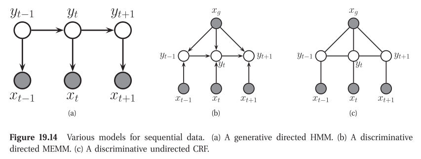
*In case the above link is broken, click here

For more CRF see this playlist, section 3.

---

Confidence Inteval and Normal Approximation

For the following procedures, the assumption is that both $np \gt 10$ and $n(1-p) \gt 10$ . When we’re constructing confidence intervals, $p$ is typically unknown, in which case we use $\hat p$ as an estimate of $p$ .

This means that our sample needs to have at least $10$ successes and at least $10$ failures in order to construct a confidence interval using the normal approximation method.

$ ss \pm m*se $

• $ss$ : sample statistics
• $m$ : multiplier
• $se$ : standard error
• $m*se$ : margin of error

The sample statistic here is the sample proportion $\hat p$, . When using the normal approximation method the multiplier is taken from the standard normal distribution (i.e., $z$ distribution). And, the standard error is computed using $\hat p$ as an estimate of $p$: $\sqrt{\frac{\hat p (1 - \hat p)}{n}}$ . This leaves us with the following formula to construct a confidence interval for a population proportion:

$ \hat{p} \pm z*(\sqrt{\frac{\hat p (1 - \hat p)}{n}}) $

Reference:

• STAT 200: PennState
• slide

---

Exercise:

1. What is Label Bias problem?
2. What is Hidden Markov Model? [murphy, sec. $10.2.2$ and ch: $17$]

---