Scalable Machine Learning

Content

Content
How to Speed up Scikit-Learn Model Training
Using the Right Processors CPUs, GPUs, ASICs, and TPUs
Distributed model training
1. Distributed Machine Learning
Scaling to trillion-parameter models
Scaling common machine learning algorithms
1. Logistic regression with 1 billion examples
Seminal Papers on Distributed Learning
Scalable Machine Learning
Tools to build large scale ML System
How to structure PySpark application
1. Debugging PySPark Application
Distributed Deep Learning
1. PyTorch Dataparallel
Guide to Scale Machine Learning Models in Production
Scalable API - Deep Learning in Production
1. First Approach:
2. Second Approach: Deep learning in production with Keras, Redis, Flask, and Apache
Exploring PUB-SUB Architecture with Redis & Python
1. What is the PUB/SUB Pattern?
2. Test Environment
Improved matrix multiplication using CUDA

How to Speed up Scikit-Learn Model Training

There are quite a few approaches to solving this problem like:

Changing your optimization function (solver)

Some solvers can take longer to converge. Image from Gaël Varoquaux’s talk.

Better algorithms allow you to make better use of the same hardware.

With a more efficient algorithm, you can produce an optimal model faster. One way to do this is to change your optimization algorithm (solver). For example, scikit-learn’s logistic regression, allows you to choose between solvers like newton-cg, lbfgs, liblinear, sag, and saga.

*In case the above link is broken, click here

*watch from $11:11$

A full gradient algorithm (liblinear) converges rapidly, but each iteration (shown as a white +) can be prohibitively costly because it requires you to use all of the data.
In a sub-sampled approach, each iteration is cheap to compute, but it can converge much more slowly.
Hybrid: Some algorithms like saga achieve the best of both worlds. Each iteration is cheap to compute, and the algorithm converges rapidly because of a variance reduction technique.

Different hyperparameter optimization techniques

To achieve high performance for most scikit-learn algorithms, you need to tune a model’s hyperparameters. Hyperparameters are the parameters of a model which are not updated during training. They can be used to configure the model or training function.

Scikit-Learn natively contains a couple techniques for hyperparameter tuning like grid search (GridSearchCV) which exhaustively considers all parameter combinations and randomized search (RandomizedSearchCV) which samples a given number of candidates from a parameter space with a specified distribution.

Recently, scikit-learn added the experimental hyperparameter search estimators halving grid search (HalvingGridSearchCV) and halving random search (HalvingRandomSearch).

There is a library called Tune-sklearn that provides cutting edge hyperparameter tuning techniques (bayesian optimization, early stopping, and distributed execution) that can provide significant speedups over grid search and random search.

Tune-sklearn is fast

Parallelize or distribute your training with joblib and Ray

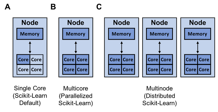
Another way to increase your model building speed is to parallelize or distribute your training with joblib and Ray.

By default, scikit-learn trains a model using a single core.

A random forest® is an easy model to parallelize as each decision tree is independent of the others.

Scikit-Learn can parallelize training on a single node with joblib which by default uses the loky backend. Joblib allows you to choose between backends like loky, multiprocessing, dask, and ray. This is a great feature as the ‘loky’ backend is optimized for a single node and not for running distributed (multinode) applications. Running distributed applications can introduce a host of complexities like:

Scheduling tasks across multiple machines
Transferring data efficiently
Recovering from machine failures

Fortunately, the Ray backend can handle these details for you, keep things simple, and give you better performance. The image below shows the normalized speedup in terms of execution time of Ray, Multiprocessing, and Dask relative to the default ‘loky’ backend.

The performance was measured on one, five, and ten m5.8xlarge nodes with 32 cores each. The performance of Loky and Multiprocessing does not depend on the number of machines because they run on a single machine.

Reference:

Using the Right Processors CPUs, GPUs, ASICs, and TPUs

CPUs are not ideal for large scale machine learning (ML), and they can quickly turn into a bottleneck because of the sequential processing nature. An upgrade on CPUs for ML is GPUs (graphics processing units). Unlike CPUs, GPUs contain hundreds of embedded ALUs, which make them a very good choice for any process that can benefit by leveraging parallelized computations. GPUs are much faster than CPUs for computations like vector multiplications. However, both CPUs and GPUs are designed for general purpose usage and suffer from von Neumann bottleneck () and higher power consumption.

von Neumann bottleneck: The shared bus between the program memory and data memory leads to the von Neumann bottleneck, the limited throughput (data transfer rate) between the central processing unit (CPU) and memory compared to the amount of memory.

A step beyond CPUs and GPUs is ASICs (Application Specific Integrated Chips), where we trade general flexibility for an increase in performance. There have been a lot of exciting research on for designing ASICs for deep learning, and Google has already come up with three generations of ASICs called Tensor Processing Units (TPUs).

TPUs exploit the fact that neural network computations are operations of matrix multiplication and addition, and have the specialized architecture to perform just that. TPUs consist of MAC units (multipliers and accumulators) arranged in a systolic array fashion, which enables matrix multiplications without memory access, thus consuming less power and reducing costs.

systolic array: In parallel computer architectures, a systolic array is a homogeneous network of tightly coupled data processing units (DPUs) called cells or nodes. Each node or DPU independently computes a partial result as a function of the data received from its upstream neighbors, stores the result within itself and passes it downstream.

This way of performing matrix multiplications also reduces the computational complexity from the order of $n^3$ to order of $3n - 2$. for more details check here.

Reference:

Distributed model training

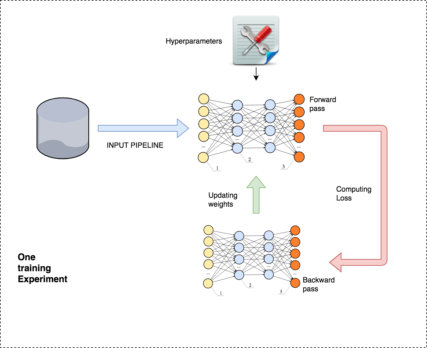
A typical, supervised learning experiment consists of feeding the data via the input pipeline, doing a forward pass, computing loss, and then correcting the parameters with an objective to minimize the loss. Performances of various hyperparameters and architectures are evaluated before selecting the best one.

Let’s explore how we can apply the divide and conquer approach to decompose the computations performed in these steps into granular ones that can be run independently of each other, and aggregated later on to get the desired result. After decomposition, we can leverage horizontal scaling of our systems to improve time, cost, and performance.

There are two dimensions to decomposition: functional decomposition and data decomposition.

Functional decomposition: Functional decomposition generally implies breaking the logic down to distinct and independent functional units, which can later be recomposed to get the results. “Model parallelism” is one kind of functional decomposition in the context of machine learning. The idea is to split different parts of the model computations to different devices so that they can execute in parallel and speed up the training.

Data decomposition: Data decomposition is a more obvious form of decomposition. Data is divided into chunks, and multiple machines perform the same computations on different data.

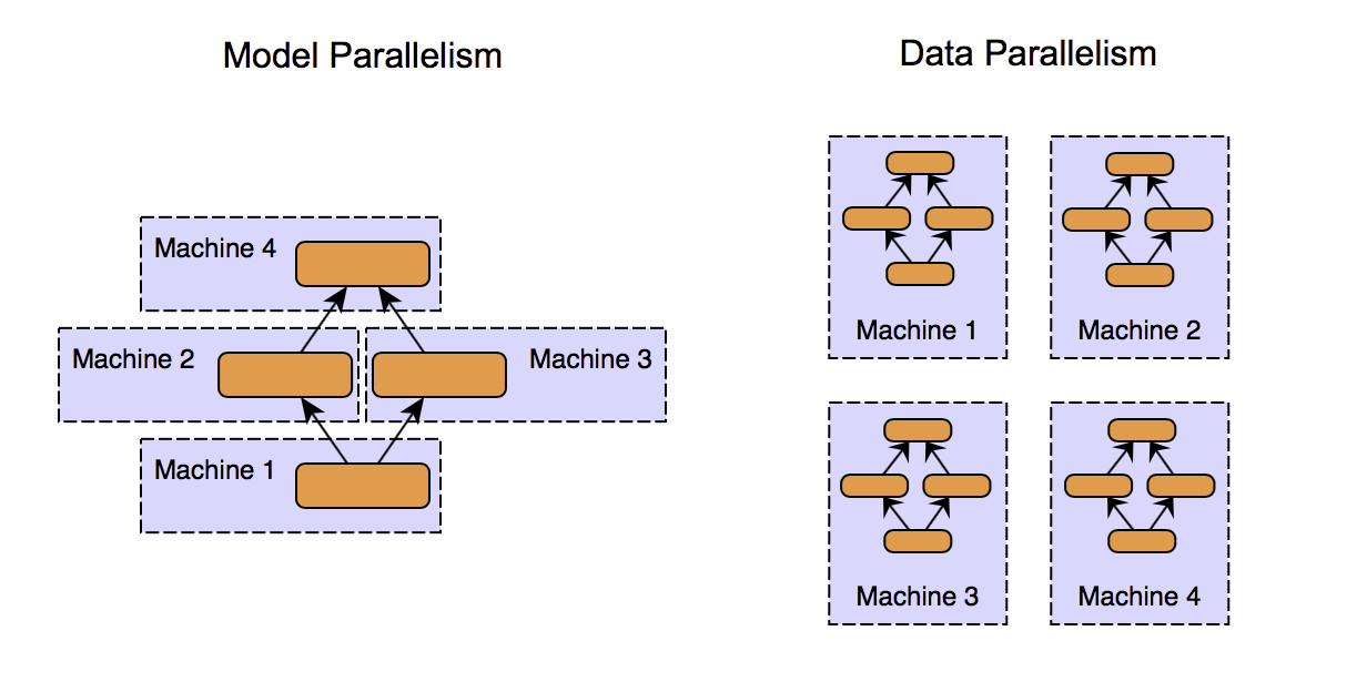
Example: One instance where you can see both the functional and data decomposition in action is the training of an ensemble learning model like random forest, which is conceptually a collection of decision trees. Decomposing the model into individual decision trees in functional decomposition, and then further training the individual tree in parallel is known as data parallelism. It is also an example of what’s called embarrassingly parallel tasks.

Distributed Machine Learning

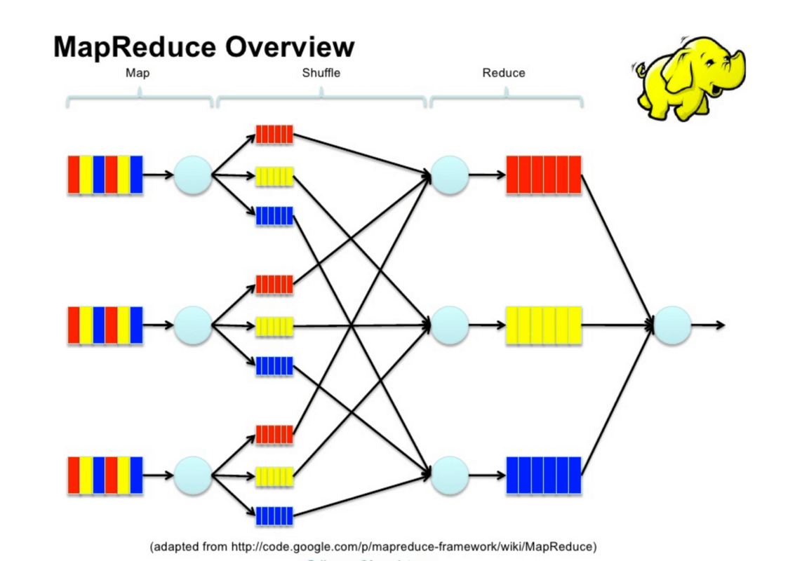
MapReduce paradigm

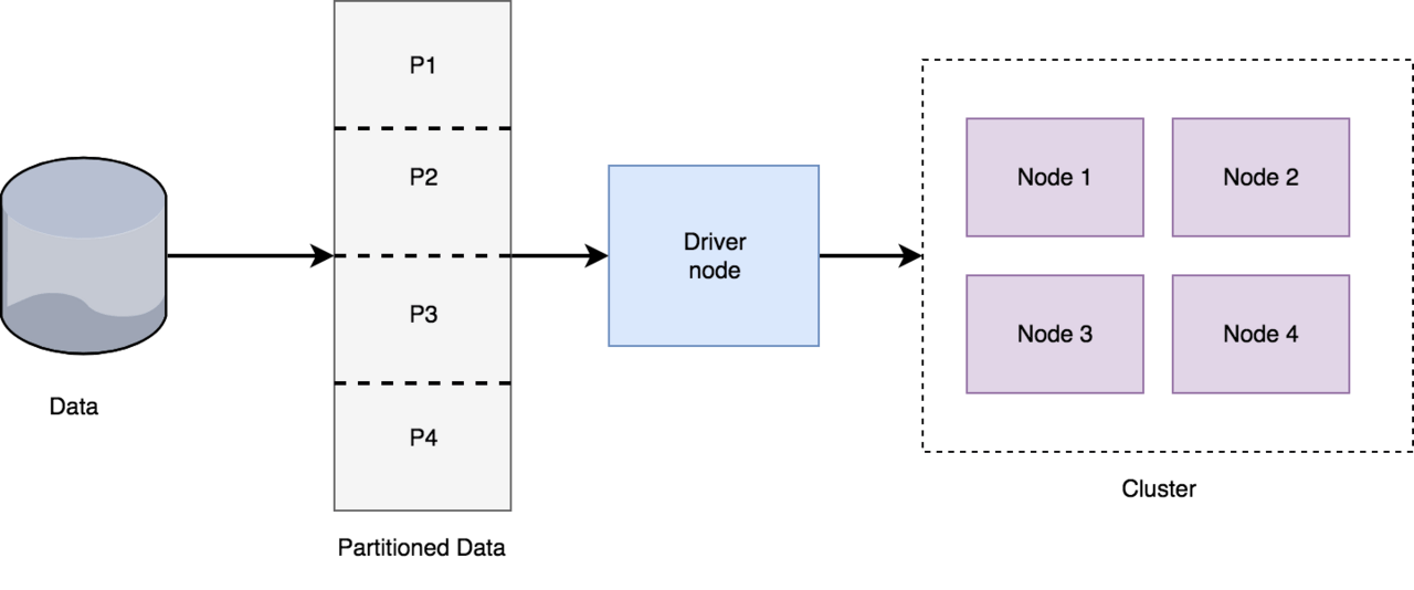
Distributed machine learning architecture

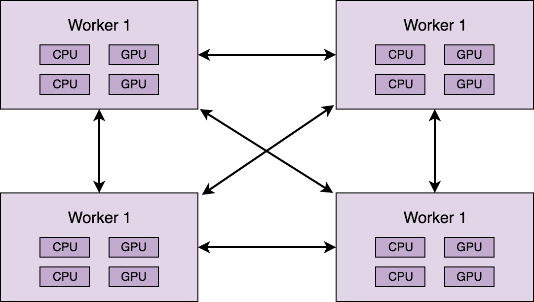
The data is partitioned, and the driver node assigns tasks to the nodes in the cluster. The nodes might have to communicate among each other to propagate information, like the gradients. There are various arrangements possible for the nodes, and a couple of extreme ones include Async parameter server and Sync AllReduce.

Async parameter server architecture

Sync AllReduce architecture

Popular frameworks for distributed machine learning

Apache Hadoop
Apache Spark
Apache Mahout

Reference:

Machine Learning: How to Build Scalable Machine Learning Models

Scaling to trillion-parameter models

With the rapid growth of compute available on modern GPU clusters, training a powerful trillion-parameter model with incredible capabilities is no longer a far-fetched dream but rather a near-future reality. DeepSpeed has combined three powerful technologies to enable training trillion-scale models and to scale to thousands of GPUs: data parallel training, model parallel training, and pipeline parallel training. This symbiosis scales deep learning training far beyond what each of the strategies can offer in isolation. 3D parallelism simultaneously addresses the two fundamental challenges toward training trillion-parameter models: memory efficiency and compute efficiency. As a result, DeepSpeed can scale to fit the most massive models in memory without sacrificing speed.

Figure 1: Example 3D parallelism with 32 workers. Layers of the neural network are divided among four pipeline stages. Layers within each pipeline stage are further partitioned among four model parallel workers. Lastly, each pipeline is replicated across two data parallel instances, and ZeRO partitions the optimizer states across the data parallel replicas.

Figure 2: Mapping of workers in Figure 1 to GPUs on a system with eight nodes, each with four GPUs. Coloring denotes GPUs on the same node.

For more details, read here

Scaling common machine learning algorithms

Logistic regression with 1 billion examples

Reference:

ML impossible: Train 1 billion samples in 5 minutes on your laptop using Vaex and Scikit-Learn

Seminal Papers on Distributed Learning

Scalable Machine Learning

Tools to build large scale ML System

How to structure PySpark application

*In case the above link is broken, click here

Debugging PySPark Application

*In case the above link is broken, click here

Distributed Deep Learning

Distributed Deep Learning Pipelines with PySpark and Keras

PyTorch Dataparallel

PyTorch has relatively simple interface for distributed training. To do distributed training, the model would just have to be wrapped using DistributedDataParallel and the training script would just have to be launched using torch.distributed.launch.

Please look at this tutorial for docker based distributed deep learning training

Resource:

Guide to Scale Machine Learning Models in Production

Hands-on example here.

Scalable API - Deep Learning in Production

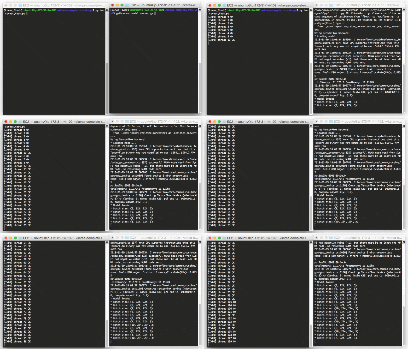
*image source

Shipping deep learning models to production is a non-trivial task

If you don’t believe me, take a second and look at the “tech giants” such as Amazon, Google, Microsoft, etc. — nearly all of them provide some method to ship your machine learning/deep learning models to production in the cloud.

This type of situation is more common than you may think. Consider:

An in-house project where you cannot move sensitive data outside your network
A project that specifies that the entire infrastructure must reside within the company
A government organization that needs a private cloud
A startup that is in “stealth mode” and needs to stress test their service/application in-house

*Please follow this amazing blog from Adrian Rosebrock from Pyimagesearch

First Approach:

A scalable Keras + deep learning REST API

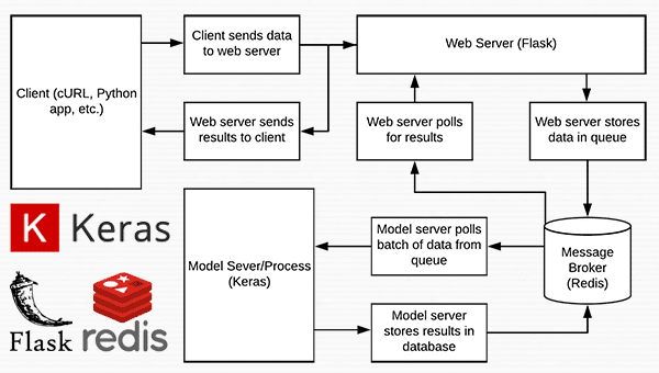
A short introduction to Redis as a REST API message broker/message queue

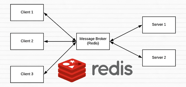
Redis is an in-memory data store. It is different than a simple key/value store (such as memcached) as it can can store actual data structures.

Memcache: Free & open source, high-performance, distributed memory object caching system, generic in nature, but intended for use in speeding up dynamic web applications by alleviating database load.

Steps:

Running Redis on our machine
Queuing up data (images) to our Redis store to be processed by our REST API
Polling Redis for new batches of input images
Classifying the images and returning the results to the client

Read the full blog and have practical experience.

Considerations when scaling your deep learning REST API

If you anticipate heavy load for extended periods of time on your deep learning REST API you may want to consider a load balancing algorithm such as round-robin scheduling to help evenly distribute requests across multiple GPU machines and Redis servers.
Keep in mind that Redis is an in-memory data store so we can only store as many images in the queue we have available memory.
A single 224 x 224 x 3 image with a float32 data type will consume $602112$ bytes of memory.
Assuming a server with a modest $16$ GB of RAM, this implies that we can hold approximately $26500$ images in our queue, but at that point we likely would want to add more GPU servers to burn through the queue faster.

Subtle issue: Multiple Model Syndrome:

Depending on how you deploy your deep learning REST API, there is a subtle problem with keeping the classify_process function in the same file as the rest of our web API code.

Most web servers, including Apache and nginx, allow for multiple client threads.

If you keep classify_process in the same file as your predict view, then you may load multiple models if your server software deems it necessary to create a new thread to serve the incoming client requests — for every new thread, a new view will be created, and therefore a new model will be loaded.

Solution: The solution is to move classify_process to an entirely separate process and then start it along with your Flask web server and Redis server. Follow second approach

Second Approach: Deep learning in production with Keras, Redis, Flask, and Apache

*Follow this amazing blog by Adrian Rosebrock from pyimagesearch and try yourself

The main idea is almost similar to first approach, but with code refactorring to avoid subtle memory issues.
Also focus on the concept of stress test.

There is a FastAPI + Docker vesion available for the second approach. Please follow this blog. Try this code.

Exploring PUB-SUB Architecture with Redis & Python

What is the PUB/SUB Pattern?

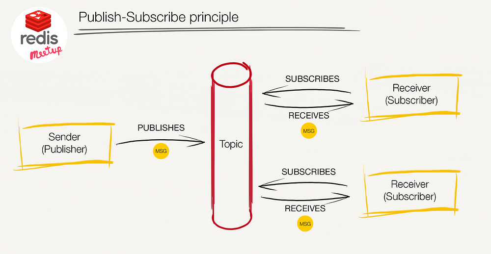
Pub/Sub aka Publish-Subscribe pattern is a pattern in which there are three main components, sender, receiver & a broker. The communication is processed by the broker, it helps the sender or publisher to publish information and deliver that information to the receiver or subscriber.

Test Environment

Start redis-server

subscriber.py

import redis
# connect with redis server as Bob
bob_r = redis.Redis(host='localhost', port=6379, db=0)
bob_p = bob_r.pubsub()

# subscribe to channel: classical music
bob_p.subscribe('classical_music')

publisher.py

# connect with redis server as Alice
alice_r = redis.Redis(host='localhost', port=6379, db=0)
# publish new music in the channel epic_music
alice_r.publish('classical_music', 'Raga Vairabi - Pt. Ajoy Chakrabarty')

By using the publish method Alice can now publish music on the classical_music Channel. Bob, on the other hand, can easily fetch publish music using the get_message() method:

# ignore Bob subscribed message
bob_p.get_message()
# now bob can find alice’s music by simply using get_message()
new_music = bob_p.get_message()['data']
print(new_music)

Reference:

Improved matrix multiplication using CUDA

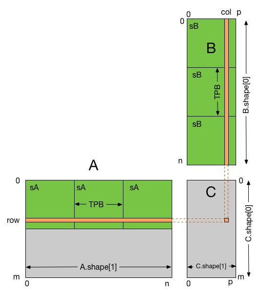
The following example shows how shared memory can be used when performing matrix multiplication.

In this example, each thread block is responsible for computing a square sub-matrix of C and each thread for computing an element of the sub-matrix. The sub-matrix is equal to the product of a square sub-matrix of A (sA) and a square sub-matrix of B (sB). In order to fit into the device resources, the two input matrices are divided into as many square sub-matrices of dimension TPB as necessary, and the result computed as the sum of the products of these square sub-matrices.

Each product is performed by first loading sA and sB from global memory to shared memory, with one thread loading each element of each sub-matrix. Once sA and sB have been loaded, each thread accumulates the result into a register (tmp). Once all the products have been calculated, the results are written to the matrix C in global memory.

By blocking the computation this way, we can reduce the number of global memory accesses since A is now only read B.shape[1] / TPB times and B is read A.shape[0] / TPB times.

matrix multiplication using shared memory

Reference:

CUDA Programming

Published on December 1, 2020