Content

1. Content
2. What is tf-idf?
3. Tf-Idf fails in document classification/clustering? How can you improve further?
4. How do you perform text classification? [ML Based Approach]
5. Naive Bayes Classification:
6. Discuss more on Language Model
7. What is LDA - Linear Discriminant Analysis
   1. Why we need LDA when we have Logistic Regression?
   2. How LDA is related to PCA?
8. Topic Modelling - LDA: Latent Dirichlet Allocation
   1. More on LDA: Latent Dirichlet Allocation
   2. Dirichlet Distribution
9. What is LSI: Latent Semantic Indexing? (or LSA)
   1. More on Latent Semantic Indexing (LSI/LSA) ?
   2. Where you can apply Latent Semantic Analysis?
   3. Pros and Cons of LSA
   4. Difference between LSI (LSA) and LDA?
10. How LDA and LSI are related?
    1. Latent Semantic Analysis (LSA) for Text Classification Tutorial?
11. What is Nonnegative Matrix Factorization (NMF) ?
    1. When do we use NMF?
12. Exercise:

---

Quick Refresher: Neural Network in NLP

What is tf-idf?

Term Frequency: we assign to each term in a document a weight for that term, that depends on the number of occurrences of the term in the document. We would like to compute a score between a query term $t$ and a document $d$, based on the weight of $t$ in $d$. The simplest approach is to assign the weight to be equal to the number of occurrences of term t in document d. This weighting scheme is referred to as term frequency and is denoted $tf_{t,d}$, with the subscripts denoting the term and the document in order.

Inverse Document Frequency:

Raw term frequency as above suffers from a critical problem: all terms are considered equally important when it comes to assessing relevancy on a query.

Rare term is more informative than the common term.

A mechanism is introduced for attenuating the effect of terms that occur too often. The idea would be to reduce the tf weight of a term by a factor that grows with its collection frequency. So it is more commonplace to use for this purpose, the document frequency $df_t$, defined to be the number of documents in the collection that contain a term $t$. We then define the inverse document frequency ($idf$) of a term $t$ as follows

$idf_t = \log \frac{N}{df_t}$

Finally, The $tf_idf$ weighting scheme assigns to term $t$ a weight in document $d$ given by:

$tf\_idf_{t,d} = tf_{t,d} * idf_t$

Content

---

Tf-Idf fails in document classification/clustering? How can you improve further?

TF-IDF is supposed to be a weighting scheme that puts more weight on more relevant keywords. And by design, it chooses those keywords as relevant which are uncommon or rare in the corpus.

The main disadvantages of using tf/idf is that it clusters documents which have more similar uncommon keywords. So it’s only good to identify near identical documents. For example consider the following sentences:

Example 1:

1. The website Stackoverflow is a nice place.
2. Stackoverflow is a website.

Two sentences from Example 1 will likely by clustered together with a reasonable threshold value since they share a lot of keywords. But now consider the following two sentences in example 2:

Example 2:

1. The website Stackoverflow is a nice place.
2. I visit Stackoverflow regularly.

Now by using tf/idf the clustering algorithm will fail miserably because they only share one keyword even though they both talk about the same topic.

And also for very short documents, like tweet, it’s difficult to rely on tf-idf score.

So one can try:

• LSI - Latent Semantic Indexing
• LDA - Latent Drichlet Allocation
• NMF - Non-negative Matrix Factorization

Currently the better solution is go with deep learning based approach. In simple from first convert the word into vector representation using any pre-trained model. And feed those vector representation in deep learning architecture.

Simple:

• Embedding Layer
• LSTM
• FC

This sort of architecture now outperforms all the traditional document clustering system.

Reference:

• better-text-documents-clustering

Content

---

How do you perform text classification? [ML Based Approach]

There are many ways to do it and those methods have evolved over time.

• Naive Bayes (Count Based Approach)
• Language Modelling (ML technique)
  • N-gram approach
  • LDA
  • LSI
• Language Modelling (DL Technique)
  • LSTM
  • RNN
  • Encoder Decoder

TODO: Review the answer

Content

---

Naive Bayes Classification:

We want to maximize the class ($c$) probability given the document $d$

$\hat c = argmax_{c \in C} P(c \vert d) = argmax_{c \in C} \frac{P(d \vert c)P(c)}{P(d)}$ $\hat c = argmax_{c \in C} P(c \vert d) = argmax_{c \in C} P(d \vert c)P(c)$

Where $P(d \vert c)$, likelihood of the data and $P(c)$ is the prior.

Now the document $d$ can be seen as a collection of features $f_1, \dots ,f_n$. Therefore we can write

$ P(d \vert c) = P(f_1, \dots ,f_n \vert c) $

Unfortunately, the above equation is still too hard to compute directly: without some simplifying assumption. And here comes the great Naive Bayes assumption which is the culprit of such naming naive.

• Assumption 1: bag of words - i.e features $f_1, \dots ,f_n$ only encode word identity but not their position.
• Naive-Bayes Assumption: The conditional independence assumption that the probabilities $P(f_i \vert c)$ are independent given the class $c$. And thus:

$ P(d \vert c) = P(f_1, \dots ,f_n \vert c) = \Pi_{i=1}^n P(f_i \vert c) $ $ \hat c = argmax_{c \in C} P(c \vert d) = argmax_{c \in C} P(c) * \Pi_{i=1}^n P(f_i \vert c) $

Now again multiplication of probabilities. So again $\log()$ is at our rescue.

$ \hat c = argmax_{c \in C} \log P(c) + \Sigma_{i=1}^n \log P(f_i \vert c) $

The beauty of the above equation is, in the log-space it’s computing the predicted class as the liner combination of the input features $f_i \in d$. And also in the log-space the prior $P(c)$ somewhat acts as regularizer.

How to train the model?

How can we learn the probabilities $P(c)$ and $P(f_i \vert c)$? Let’s first consider the maximum likelihood estimate. We’ll simply use the frequencies in the data.

To learn the probability $P( f_i \vert c)$, we’ll assume a feature is just the existence of a word in the document’s bag of words, and so we’ll want $P(w_i \vert c)$.

We will use smoothing technique to avoid any zero-count problem.

Remember: Naive-Bayes is an Generative Classifier where as Logistic-Regression is an Discriminative Classifier.

Reference:

• Book: Speech and Language Processing, Jurafski, ch 4

Content

---

Discuss more on Language Model

In language model we assign a probability to each possible next word. The same model will also serve to assign probability to an entire sentence. Assigning probabilities to sequence of words is very important.

• Speech recognition
• Spelling correction
• Grammatical error correction
• Machine translation

One way to estimate probability is: relative frequency count.

Say sentence $S = w_1 w_2 w_3$ where $w_i$ are words. Then

$P(w_3 \vert w_1 w_2) = \frac{C(w_1 w_2 w_3)}{C(w_1 w_2)}$

i.e count number of times $w_3$ is used followed by $w_1 w_2$: $C(w_1 w_2 w_3)$. And divide this by how many times $w_1 w_2$ appear together $C(w_1 w_2)$.

However count based methods have flaws. New sentences are created very often and we won’t always be able to count entire sentences. For this reason, we’ll need to introduce cleverer ways of estimating the probability of a word $w$ given a history $h$, or the probability of an entire word sequence $W$.

So we can compute the probabilities of the entire sentence $S=w_1 \dots w_n$ like this:

$ P(x_1 \dots x_n) = P(x_1)P(x_2\vert x_1)P(x_3\vert x_1^2)\dots P(x_{n}\vert x_1^{n-1}) $ $ P(w_1^n)=\Pi_{k=1}^n P(x_k \vert x_1^{k-1}) $

where $x_1^n$ means $x_1 x_2 \dots x_n$. The chain rule shows the link between computing the joint probability of a sequence and computing the conditional probability of a word given previous words.

The intuition of the n-gram model is that instead of computing the probability of a word given its entire history, we can approximate the history by just the last few words. And applying Markov Assumption we can say that probability of $w_n$ depends on the previous word $w_{n-1}$ only i.e $p(w_n \vert w_{n-1})$ and thus we create the foundation of the Bi-gram model.

Now product form of so many probabilities are going to be very small. So we can take $\log()$ of $p(w_1^n)$ and get a nice summation form:

$ \log(p(w_1^n)) = \Sigma_{k=1}^{n} p(w_n \vert w_{n-1}) $

note: the above formulation is for Bi-gram model

Now interestingly the above equation gives us the joint probability of those words together. So, it’s showing the likelihood (i.e. the probability) of the data (i.e. the sentence). To estmiate these likelihood we can go for maximization $\rightarrow$ Maximum Likelihood Estimation.

Evaluation: In practice we don’t use raw probability as our metric for evaluating language models, but a variant called perplexity. However the concept of perplexity is related to entropy. [For more details look here]

There is another way to think about perplexity: as the weighted average branching factor of a language. The branching factor of a language is the number of possible next word that can follow any word.

However with count based approach we may face the situation of Zero Count problem. And to mitigate that use Smoothing.

Smoothing:

• Laplace Smoothing (additive smoothing)
• Add-k Smoothing
• Kneser-Ney Smoothing (best one, most commonly used)
  • Kneser-Ney smoothing makes use of the probability of a word being a novel continuation. The interpolated Kneser-Ney smoothing algorithm mixes a discounted probability with a lower-order continuation probability.

Reference:

• Book: Speech and Language Processing, Jurafski, ch 3,

Content

---

What is LDA - Linear Discriminant Analysis

… model the distribution of the predictors $X$ separately in each of the response classes $Y$…

• Logistic regression involves directly modeling $P(Y = k \vert X = x)$ using the logistic function. But in LDA we take indirect approach. In this alternative approach, we model the distribution of the predictors $X$ separately in each of the response classes (i.e. given $x$), and then use Bayes’ theorem to flip these around into estimates for $Pr(Y = k \vert X = x)$.
• When these distributions are assumed to be normal, it turns out that the model is very similar in form to logistic regression.

Why we need LDA when we have Logistic Regression?

• Stability when well separated: When the classes are well-separated, the parameter estimates for the logistic regression model are surprisingly unstable. Linear discriminant analysis does not suffer from this problem.
• Stability when normally distributed: If $n$ is small and the distribution of the predictors $X$ is approximately normal in each of the classes, the linear discriminant model is again more stable than the logistic regression model.
• Stability for $\gt2$ classes: Linear discriminant analysis is popular when we have more than two response classes.

How LDA is related to PCA?

Linear Discriminant Analysis (LDA) is most commonly used as dimensionality reduction technique in the pre-processing step for pattern-classification

• The goal of an LDA is to project a feature space (a dataset $n$-dimensional samples) onto a smaller subspace $k$ (where $k \leq n−1$) while maintaining the class-discriminatory information.
• It’s a classification algorithm.
• Linear Discriminant Analysis (LDA) is most commonly used as dimensionality reduction technique in the pre-processing step for pattern-classification and machine learning applications. The goal is to project a dataset onto a lower-dimensional space with good class-separability in order avoid overfitting (curse of dimensionality) and also reduce computational costs.
• The general LDA approach is very similar to a Principal Component Analysis. LDA tries to satisfy the below $2$ conditions:
  • Dimensionality Reduction: Find component axes that maximizes the variances (similar to PCA).
  • Class Separability: Find axes that maximizes the separation between multiple classes.

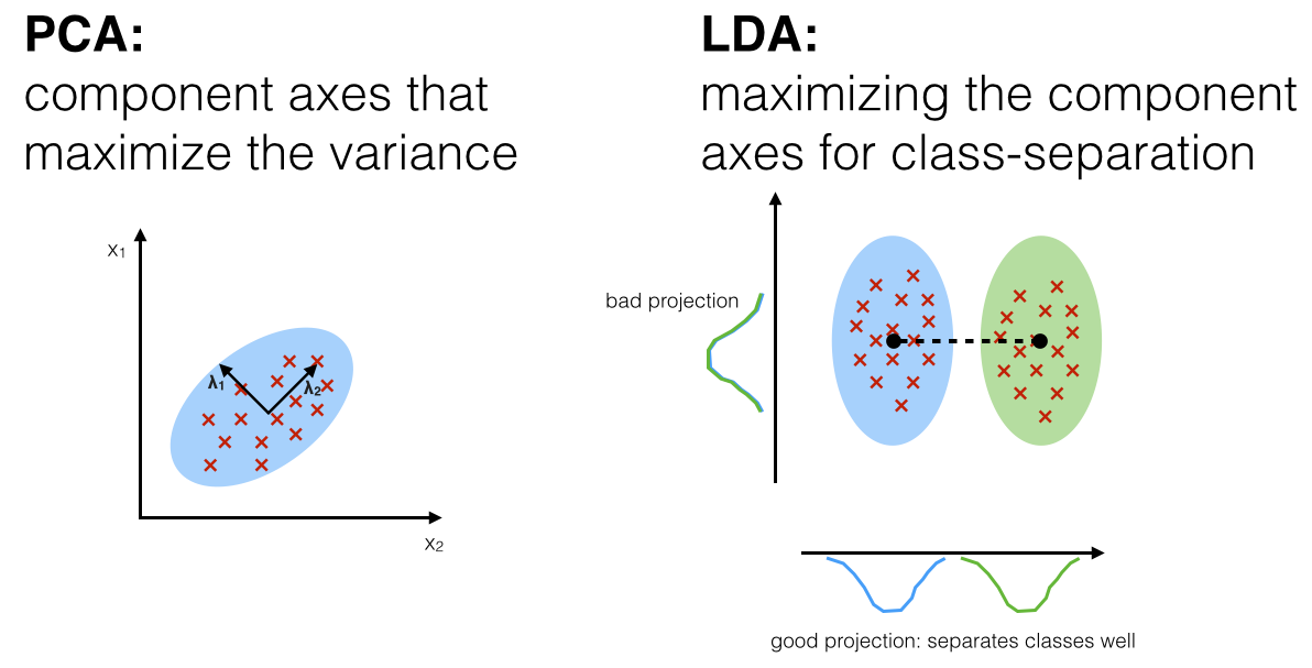
• Both Linear Discriminant Analysis (LDA) and Principal Component Analysis (PCA) are linear transformation techniques that are commonly used for dimensionality reduction.
• PCA is unsupervised where as LDA is supervised and LDA computes the directions (linear discriminants) that will represent the axes that maximize the separation between multiple classes

Reference:

• Sebastian Raschka
• Book: ISL, Chapter 4
• Lecture 9: Stat202

Content

---

Topic Modelling - LDA: Latent Dirichlet Allocation

…a repeating pattern of co-occurring terms in a corpus…

Topic Modelling is different from rule-based text mining approaches that use regular expressions or dictionary based keyword searching techniques. It is an unsupervised approach used for finding and observing the bunch of words (called topics) in large clusters of texts.

Topics can be defined as a repeating pattern of co-occurring terms in a corpus. A good topic model should result in

• health, doctor, patient, hospital for a topic $\rightarrow$ Healthcare
• farm, crops, wheat for a topic $\rightarrow$ Farming.

Topic Models are very useful for the purpose for

• Document clustering
• Organizing large blocks of textual data
• Information retrieval from unstructured text
• Feature selection.

Application:

• News Recommendation: New York Times are using topic models to boost their user – article recommendation engines.
• Candidate Recruitment from CV: Various professionals are using topic models for recruitment industries where they aim to extract latent features of job descriptions and map them to right candidates.

They are being used to organize large datasets of emails, customer reviews, and user social media profiles.

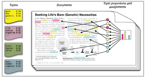
You can try doing topic modelling using the following methods.

• Term Frequency and Inverse Document Frequency.
• Non negative Matrix Factorization (NMF)
• LDA - Latent Dirichlet Allocation

Performance vs Accuracy: NMF is supposed to be a lot faster than LDA, but LDAs supposed to be more accurate. Problem is LDA takes a long time, unless you’re using distributed computing.

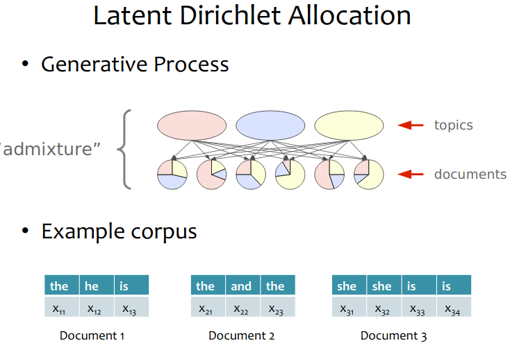
Assumption: LDA assumes documents are produced from a mixture of topics. Those topics then generate words based on their probability distribution.

Given a dataset of documents, LDA backtracks and tries to figure out what topics would create those documents in the first place.

LDA is a probabilistic matrix factorization technique.

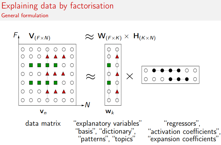
In vector space, any corpus (collection of documents) can be represented as a document-term matrix. Matrix Factorization converts this Document-Term Matrix ($N \times M$) into two lower dimensional matrices – $M_1$ and $M_2$.

• $M_1$ is a document-topics matrix ($N \times K$)
• $M_2$ is a topic – terms matrix ($K \times M$)

where

• $N$ is the number of documents
• $K$ is the number of topics
• $M$ is the vocabulary size.

It iterates through each word $w_i$ for each document $d_j$ and tries to adjust the current topic – word assignment with a new assignment. A new topic $t_k$ is assigned to word $w_i$ with a probability $p$ which is a product of two probabilities $p_1$ and $p_2$.

For every topic, two probabilities $p_1$ and $p_2$ are calculated.

• $p_1$: $p(t_k \vert d_j)$ = the proportion of words in document $d_j$ that are currently assigned to topic $t_k$.
• $p_2$: $p(w_i \vert t_k)$ = the proportion of assignments to topic $t_k$ over all documents that come from this word $w_i$.

The current topic – word assignment is updated with a new topic with the probability, product of $p_1$ and $p_2$ .

Assumption: The model assumes that all the existing word – topic assignments, except the current word are correct. This is essentially the probability that topic $t_k$ generated word $w_i$, so it makes sense to adjust the current word’s topic with new probability.

After a number of iterations, a steady state is achieved where the document-topic and topic-term distributions are fairly good..

References:

• AVB <- Wrongly says LDA is MF. LDA is actutally probabilistic MF.
• EdwinChen
• medium-PySparkImplementation

Content

---

More on LDA: Latent Dirichlet Allocation

• Generative model for topic modelling. It’s an unsupervised learning.
• LDA is one of the early versions of a topic model which was first presented by David Blei, Andrew Ng, and Michael I. Jordan in 2003.
• In essence, LDA is a generative model that allows observations about data to be explained by unobserved latent variables that explain why some parts of the data are similar, or potentially belong to groups of similar topics.

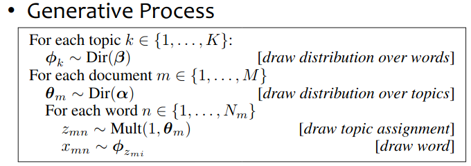
Each doccument is a mixture of topic:

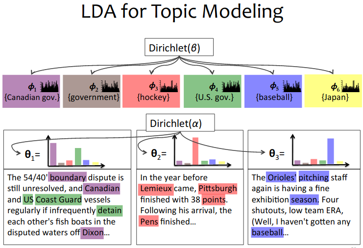
• Originally presented in a graphical model and using Variational Inference
• Builds on latent semantic analysis
• It is a mixed-­membership model.
• It relates to PCA and matrix factorization

The generative story begins with begins with only Dirichlet Prior over the topics.

Dirichlet Distribution

• In probability and statistics, the Dirichlet distribution (after Peter Gustav Lejeune Dirichlet), often denoted $Dir( \alpha )$, is a family of continuous multivariate probability distributions parameterized by a vector $\alpha$ of positive reals.
• It is a multivariate generalization of the beta distribution, hence its alternative name of multivariate beta distribution (MBD).
• Dirichlet distributions are commonly used as prior distributions in Bayesian statistics, and in fact the Dirichlet distribution is the conjugate prior of the categorical distribution and multinomial distribution.

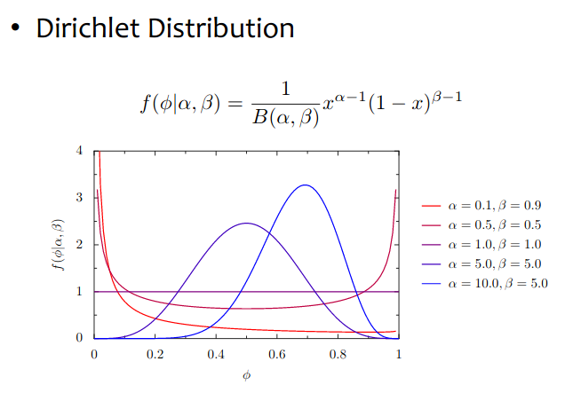
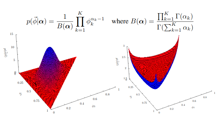
Resource:

• IMP: Topic Model: CMU
• Lecture 10: LDA
• Dirichlet_distribution

Content

---

What is LSI: Latent Semantic Indexing? (or LSA)

• LSI is also known as Latent Semantic Analysis (LSA)
• It’s SVD used in information retrieval.

The term-document matrix is the basis for computing the similarity between document and query. Can we transform this matrix so that we can get better measure of similarity between document and query?

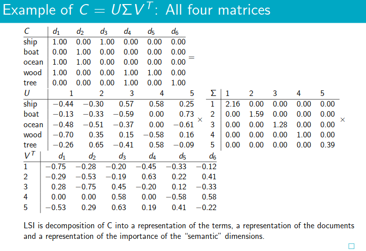
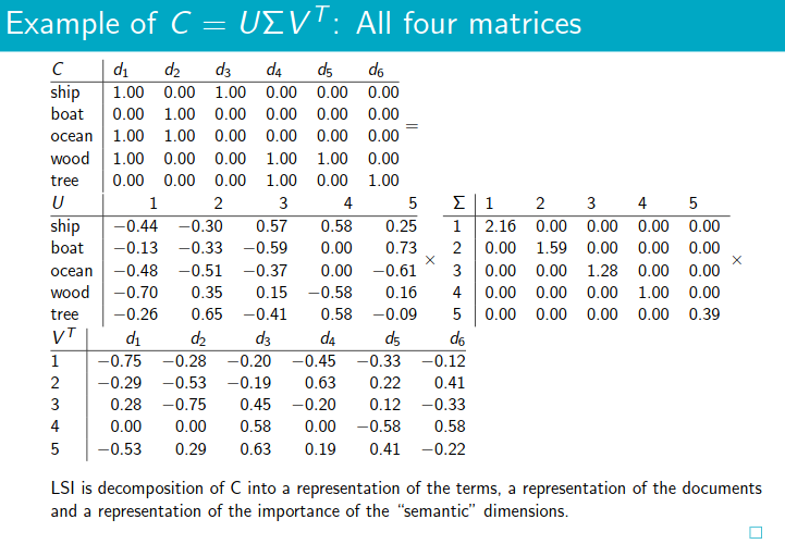
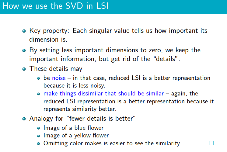
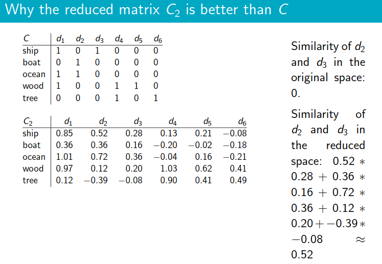
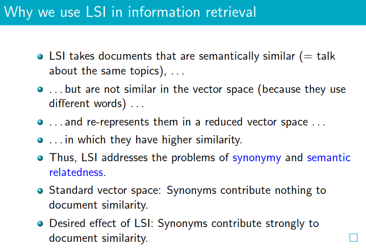
• The boat and ship are similar in meaning. The reduced similarity measure reflects this.

Reference:

• Book: Introduction to Information Retrieval by Manning, Ch 18
• Slide

Content

---

More on Latent Semantic Indexing (LSI/LSA) ?

• Latent semantic indexing is a mathematical technique to extract information from unstructured data. It is based on the principle that words used in the same context carry the same meaning.

Latent Semantic Analysis (LSA) is a theory and method for extracting and representing the contextual-usage meaning of words by statistical computations applied to a large corpus of text.

• In order to identify relevant (concept) components, or in other words, aims to group words into classes that represent concepts or semantic fields, this method applies Singular Value Decomposition to the Term-Document matrix tf-idf. As the name suggests this matrix consists of words as rows and document as columns.
• LSA itself is an unsupervised way of uncovering synonyms in a collection of documents.

Where you can apply Latent Semantic Analysis?

• Text classification
• Topic Modelling

Pros and Cons of LSA

Latent Semantic Analysis can be very useful as we saw above, but it does have its limitations. It’s important to understand both the sides of LSA so you have an idea of when to leverage it and when to try something else.

Pros:

• LSA is fast and easy to implement.
• It gives decent results, much better than a plain vector space model.

Cons:

• Since it is a linear model, it might not do well on datasets with non-linear dependencies.
• LSA assumes a Gaussian distribution (see later) of the terms in the documents, which may not be true for all problems.
• LSA involves SVD, which is computationally intensive and hard to update as new data comes up.

Reference:

• Blog
• Stepwise guide to Topic Modelling

Content

---

Difference between LSI (LSA) and LDA?

LSA was introduced in 2005 whereas LDA was introduced in 2003 .

LSI (also known as Latent Semantic Analysis, LSA) learns latent topics by performing a matrix decomposition (SVD) on the term-document matrix. It’s an upsupervised approach.

LDA is a generative probabilistic model, that assumes a Dirichlet prior over the latent topics.

LSI is much faster to train than LDA, but has lower accuracy.

LSI is a variant of PCA. LSI has a probabilistic variant developed by Thomas Hofmann known as Probabilistic latent semantic analysis, (PLSI or PLSA), which was the motivation for developing LDA. LDA is the Bayesian version of PLSI.

Reference:

• Quora

Content

---

How LDA and LSI are related?

• LSA is applying SVD on term-document matrix

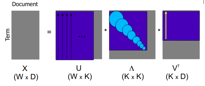
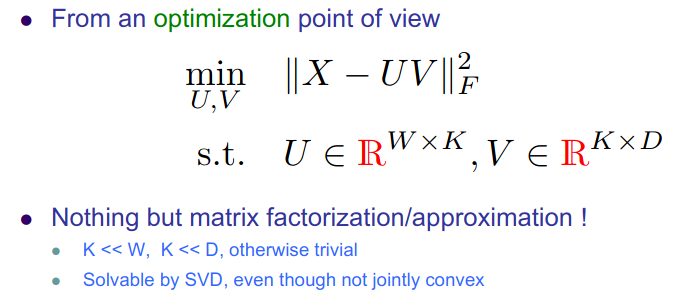
This MF (matrix factorization) technique can be molded into Probabilistic model.

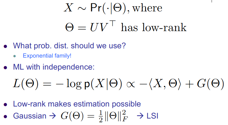
As mentioned earlier, LSI assumes Gaussian Distribution of terms in the document.

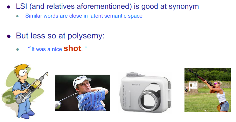
LSI is good at synonymy but bad at polysemy

Probabilistic LSI (PLSI)

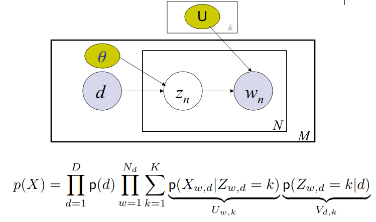
See, how term-topic matrix $U_{w,k}$ and document-topic matrix $V_{d,k}$ are included in the equation.

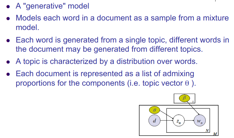
Example:

• Topic $t_1$ generates $n$ words $w_1^1, \dots, w_n^1$ and topic $t_2$ generates $n$ words $w_1^2, \dots, w_n^2$.
• Now say document $D$ has $p$ words from topic $t_1$ and $q$ words from topic $t_2$ s.t $D=[w_1^1, \dots, w_p^1, w_1^2, \dots, w_q^2]$
• Thus document $D$ is mixture of topic $t_1$ and $t_2$.

Say there is a movie on cricket. And then there is a movie review available in IMDB. In movie related documents, we will see words like [director, producer, actor, award, songs, dialogue] and in cricket related documents we will see words like [cricket, player, bat, ball, run, batsman, bowler, $\dots$]

*image source

This movie review has words from both topic movie and cricket

coming back to PLSI…

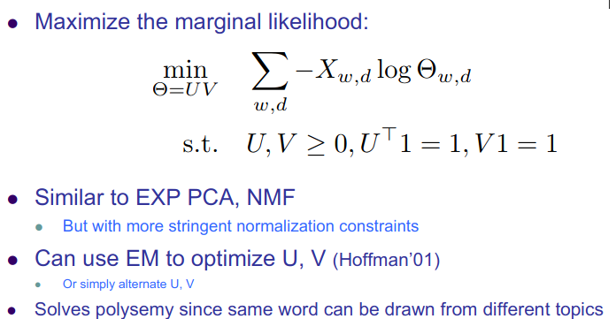
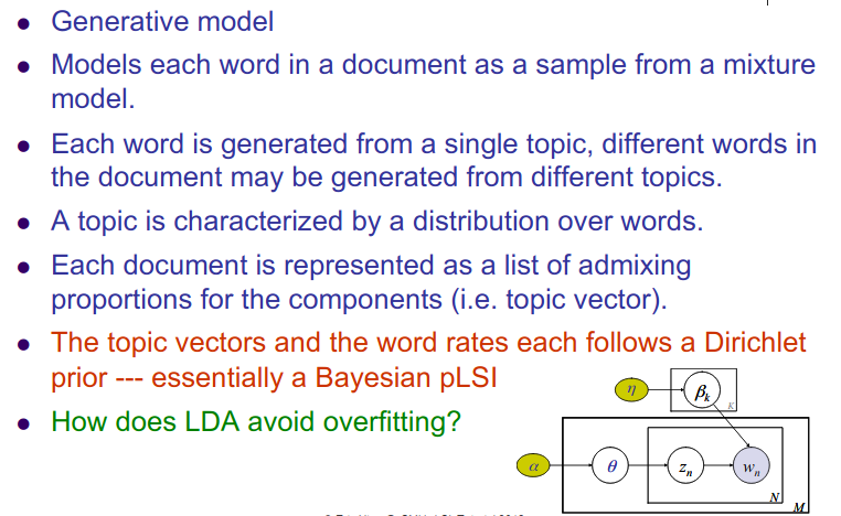
Latent Drichlet Allocation is a Bayesian PLSI. BAM !!

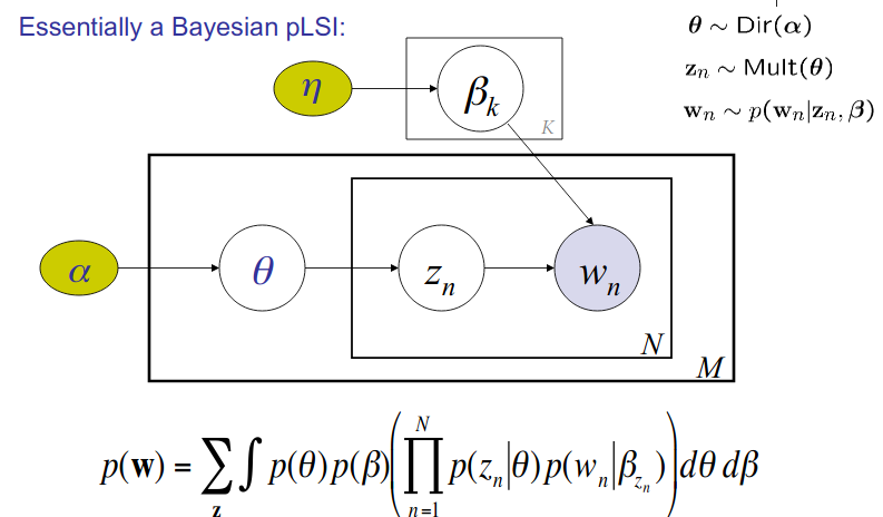
memorize the equation

LDA can also be modeled as Probabilistic PCA (PPCA) DOUBLE BAM !!

For more on PPCA, check slide 20 here

Summary:

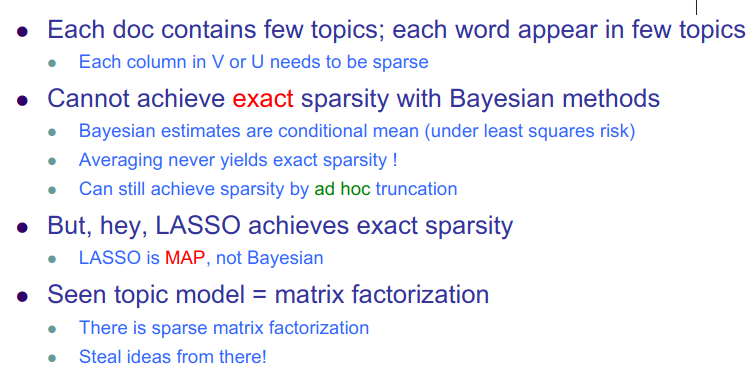
Bonus: How Sparsity works here?

Reference:

• CMU Slide

---

Latent Semantic Analysis (LSA) for Text Classification Tutorial?

• AV

---

What is Nonnegative Matrix Factorization (NMF) ?

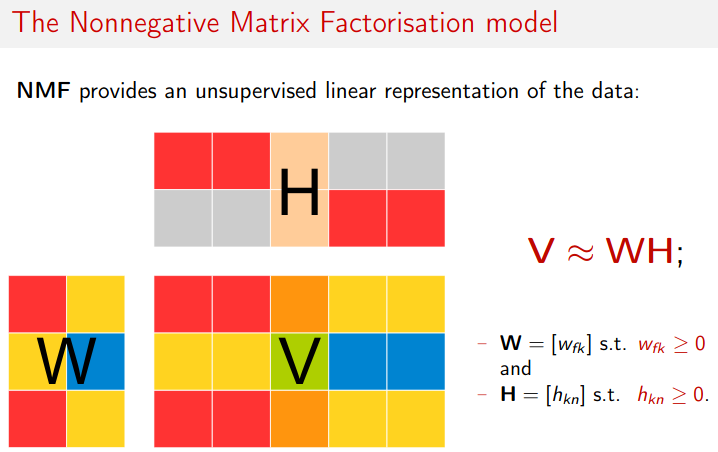
With the rise of complex models like deep learning, we often forget simpler, yet powerful machine learning methods that can be equally powerful. NMF (Nonnegative Matrix Factorization) is one effective machine learning technique that I feel does not receive enough attention. NMF has a wide range of uses, from topic modeling to signal processing.

When do we use NMF?

Example: Computer Vision

• A different, commonly used factorization method is PCA (Principle Components Analysis). But PCA creates factors that can be both positive and negative.

Let’s see what happens when we try decomposing various faces. In the following image, we show the components (bases) we calculated with PCA on the left and the weights corresponding to a single image on the right. Red represents negative values.

If you look at the components, you see that they don’t make much sense. It’s also difficult to interpret what it means for a face to have a negative component.

Now, let’s see what happens when we use NMF.

Now, the components seem to have some meaning. Some of them look like parts of a nose or parts of an eye. We can consider each face to be an overlay of several components. This means we can interpret the decomposition of a face as having a certain weight of a certain nose type, a certain amount of some eye type, etc.

Example 2: Topic Modeling

Imagine if you wanted to decompose a term-document matrix, where each column represented a document, and each element in the document represented the weight of a certain word (the weight might be the raw count or the tf-idf weighted count or some other encoding scheme; those details are not important here).

NMF decomposition of the term-document matrix would yield components that could be considered topics, and decompose each document into a weighted sum of topics. This is called topic modeling and is an important application of NMF.

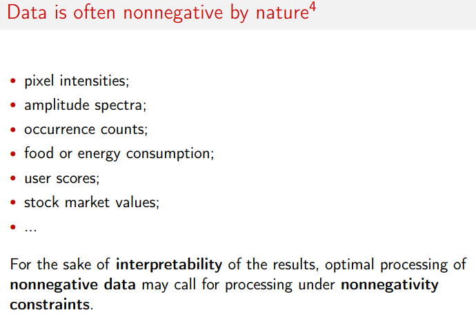
NMF ensures that after decomposition the values are non-negative, which brings lots of meaningful insight which wouldn’t have been possible in other decomposition.

Example 2: Recommendation System

• NMF in Recommendation System

Reference:

• mlexplained: nmf
• IMP NMF-tutorial

Content

---

Exercise:

1. NMF in nlp?
2. Using traditional ML, how to learn context?

---

Back to Top